 Fie:
Fabrication d’imagerie extraordinaireFie:
Fabrication d’imagerie extraordinaire
Fie:
Fabrication d’imagerie extraordinaireFie:
Fabrication d’imagerie extraordinaireTable of contents

Fie is a programme for various image-editing and related tasks. Its main purpose these days is for 3-D image segmentation, especially for the creation of 3-D models for visualization, 3-D printing, and finite-element analysis.
The usual workflow for image-based modelling is to
There are two primary design goals for Fie. First, the model geometry should remain faithful to the images. Second, if the image segmentation needs to be modified, it should be possible to generate a complete new model automatically, in one operation, without having to repeat the usual steps of repair, smoothing, volume mesh generation, and specification of physical properties. This is possible with Fie because the physical properties (e.g., colours, transparency, material properties, boundary conditions, loads) are all specified at the image-segmentation stage; and the smoothing, topological consistency and connectivity are also all established at the image-segmentation stage.
An important secondary goal is that it is easy to generate variants of a model from the same image segmentation, incorporating different component subsets and with different visual and physical properties and even different geometries.
The drawing operations in Fie can be used to trace structure outlines in stacks of images. The outlines are maintained in text files suitable for subsequent surface triangulation using Tr3, for either visualization or finite-element simulation.
The use of open contours (in addition to the usual closed contours) facilitates the controlled handling of complex structures with shared surfaces. An important feature is that one can specify that a line should start and/or finish at the start or finish of some other line. This provides a mechanism for specifying and ensuring topological continuity and integrity. This continuity is specified for a particular line within groups of slices, and is displayed graphically, so the user can visually verify connections. Since the connectivity often changes from slice to slice, a mechanism is provided to specify Joins across such divisions, and Caps can be defined to close the beginnings and ends of 3-D surfaces.
The .tr3 file produced by Fie can contain
specifications for
colours and transparency (for visualization), and also
mechanical properties, boundary conditions and loads
(for finite-element simulation), together with the
basic geometry.
Multiple subsets of a model can be defined, to generate multiple versions of a model containing different combinations of structures with different attributes or different mesh resolutions.
Triangulated models are generated in both VRML and JSON formats for interactive visualization, and in SAP format for finite-element simulation. The VRML files can be viewed using Thrup’ny or some other VRML viewer; the JSON files are designed to be viewed using Thrwp’ny, a 3-D viewer based on JavaScript and WebGL. The SAP finite-element model files can be converted to other finite-element formats using Fad.
Descriptive texts and labels can be defined, suitable for both debugging and teaching purposes.
Alignment operations are available for aligning histological serial sections for subsequent segmentation and 3-D reconstruction.
Additional features include:
Fie is implemented in Fortran. It was originally developed under VMS and later under Unix for Alpha. It is currently being developed under Debian GNU/Linux for x86 and x86_64, and (alas) under Microsoft Windows; the binaries are available for downloading below. It can be used for any purpose as long as I am informed of its use. So far there is no documentation beyond what you’re looking at.
Fie has been evolving gradually since 1989. It was originally used for image viewing and editing. Around 1995 it absorbed features from Dig, a programme that I had been developing since 1976 for digitizing images and doing reconstruction from serial sections.
The ‘F’ originally stood for Fancy or Fortran or Funnell, depending on the phase of the moon and other factors; these days maybe it would stand for Funky. The ‘IE’ stood for Image Editor. These days we don’t use Fie much for image editing, but more for creating 3-D models, so I came up with Fabrication d’imagerie extraordinaire as a new excuse for the name Fie.
Section 2 explains how to install the software. Section 3 gives some general information about the graphical user interface, file saving and automatic backups. Section 4 contains a tutorial that is intended for self-teaching.
Section 5 presents the functions of every menu and submenu.
Section 6 then describes the detailed format of the
.tr3 file produced by Fie.
Although the file is created and
modified using Fie’s menus, there are some sections
(e.g., subset specifications) in which some of the syntax
needs to be created and edited directly by the user.
The .tr3 file is a plain-text and in
exceptional circumstances it may be desirable to examine or
even edit it with a text editor.
Section 7 presents an example to illustrate some of the features of Fie.
When new information is added to this documentation, it may be flagged as being new, like this.
If your computer is part of the McGill BME network, create a
symbolic link (ln -s) to the executable on
probeShare. Otherwise download the Fie executable from here into
a directory called Downloads in your home directory.
If you don’t already have a Downloads
directory, give the command mkdir ~/Downloads.
You may prefer to create and use ~/bin
(for ‘binary’ executable files) instead of
~/Downloads.
If you have downloaded Fie before and are trying to download a new version from here, and you seem to always get the previous version, you may need to clear the cache of your Web browser.
To make Fie executable, you can open a terminal window
(in some versions of Linux, by doing
),
and do
cd ~/Downloads
chmod u+x fie
Alternatively, you can right-click on the file in a
file-browsing window, select and
then the tab, and check
the box .
Problems:
You can run Fie by opening a terminal window and giving the command
./Downloads/fie& or, if you have already cd’d
into the Downloads directory, just ./fie&.
The & causes Fie to run in the background so your terminal
window can be used to do other things (e.g., to run Tr3) while
Fie is still running.
(By default, double-clicking on Fie in a directory listing
probably won’t work.
An alternative is to set up a custom application launcher in the top panel
of your Linux GUI, if there is such a panel.)
The MS Windows version of Fie is usually out of date, and it often behaves badly because it is built under MS Windows XP. It is strongly recommended that the Linux version of Fie be used. One approach is to install VirtualBox under Windows and then install Debian Linux under VirtualBox.
Either download the Fie executable for 32-bit Windows (about 1.5 Mbytes) or (if your computer is part of the McGill BME network) create a shortcut to the executable on probeShare. Follow the general instructions for installation of Dip software.
If you are using a copy of Fie installed on your local hard disk,
then you must also provide the Glib library and two
associated libraries. Download the following DLL files into the same
directory that fie.exe is in:
Fie has been used with MS Windows 95, 98, NT, 2000, XP, Vista, 7, 8 and 10.
Under Windows 7 and higher,
some things act strangely and sometimes the programme
fails to start. If it fails with a message that refers
to a HOME environment variable, it means that you need to
follow the instructions for setting up such a variable
(see installation of Dip software as
mentioned above). If other error messages occur upon startup,
or if text messages overwrite one another, just
try running Fie again.
There is no Mac version of Fie. One approach is to install VirtualBox under Mac OS and then install Debian Linux under VirtualBox.
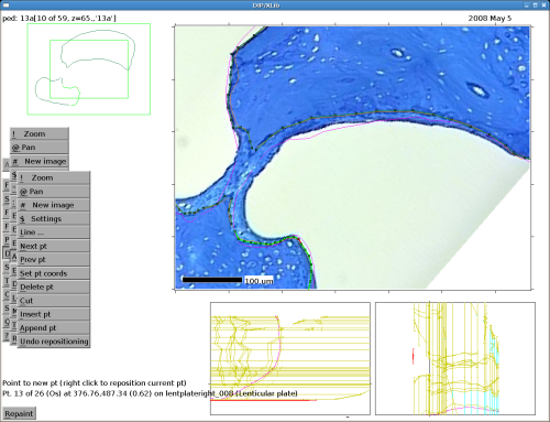
Fie has a menu-based graphical user interface. The interface is identical under different operating systems. As shown at right, the interface consists of
Fie will initially set its overall window size by trying to estimate how much screen space is available to it. You can use the function to adjust the window size by trial and error until it takes a little less than the whole vertical space available. Make sure you can see the button at the bottom of the screen, as shown in the figure.
You can adjust the font size by using the function .
See the Dip documentation for a general discussion of how to use the menus. Note that every menu button has a shortcut key, indicated by underlining in the button label.
In some cases when a menu is displayed in Fie, you can either
click on one of the menu items or click in one of the image windows.
For example, when selecting a line for some purpose, you can either click
on the appropriate button in the menu or click near the line within
either the main image window or the overview window.
When Fie saves a file, if a file already exists with the same name
then the old file is renamed by adding a version number. The version
number is of the form #n# and is appended to the
file name. For example, if three versions of the file
test.tr3 exist, called test.tr3#1#,
test.tr3#2# and test.tr3, when a new version
is saved it will be called test.tr3 and the previous
version will be renamed to test.tr3#3#.
If you ever need to recover an older version, just use your operating system to delete the later version (or rename it to something else if you’re not sure) and then rename the version you want by removing the version number.
As you are doing operations (or
operations)
Fie will automatically back up the
.tr3 file from time to time. The backup is done to a file called
fie_tr3.tmp in your HOME directory. If something goes wrong
during a session (e.g., Fie crashes or your computer crashes), or
you accidentally quit without saving your latest changes,
you can recover the contents of the
last automatic backup:
fie_tr3.tmp from
your HOME directory to the directory where your .tr3 file normally
resides.
fie_tr3.tmp to have the name of your normal .tr3 file.
The frequency with which automatic backups are done can be controlled by the item in the settings menu (which is available from within several menus). Specify how many interactive operations you want to have happen between backups.
Error messages are typically displayed near the bottom of the screen, preceded by an button. If the error message is too long to fit across the width of the Fie window, you may be able to view the entire message in a log file
Fie produces a log file named fie_log.tmp in
your home directory.
This section is intended to lead a new user through a logical succession of the tasks involved in segmenting stacks of images like X-ray CT scans, MR scans, serial-section histology or optical-sectioning microscopy.
It is assumed that you have already successfully installed Fie and have read the Introduction and the section on the User interface. It is strongly suggested that, as you go through the tutorial, you follow the provided links to the detailed documentation.
.tr3 file,
Fie creates a backup version with
a version number, so you can retrieve older versions. Fie also creates
an automatic backup file periodically, which
may be useful for getting yourself out of trouble if you haven’t saved
recently.
kill command. If you ran Fie from
within a terminal window, you should see a message
saying that you should use the menu to quit.
If you are desperate, you should be able to kill Fie
using the kill -9 command or
Ctrl\.
Fie’s favourite way of dealing with stacks of images is as collections of JPEG or PNG files. Every file in the collection must be of the same type (e.g., 8-bit grey-scale or 24-bit colour) and have the same number of pixels. The file names should follow the rules mentioned in the General notes and each file name should end in the sequence number of the image, with leading zeroes if appropriate (e.g., 001, 002, …, 150).
/media/… if you chose automatic mounting).
To follow this tutorial, download
16885.zip. Unzip the files into
some directory. There will be a directory 16885/
containing a 00readme.txt file and a jpg/
subdirectory containing 340 image files corresponding to the
human-ear magnetic-resonance microscopy (MRM)
dataset 16885 from the lab of
Drs. O.W. Henson, Jr. and Miriam M. Henson
at UNC.
The 00readme.txt
file contains the voxel size for the dataset.
To create a new .tr3 file for a set of images,
start by clicking on
and then
and then
.
You will be asked whether you have a set of .jpg or .png files.
If you click on
the operation will be cancelled.
For this tutorial,
click on .
You will now see a menu for browsing, and a message telling you to
Specify first image file. Unless the file already appears
in the menu, browse to find it.
Once you have selected
the first image in your series, you will be asked to
Specify last image file. Browse and select the last image
in your series. Fie will try to determine the number of digits in the
sequence numbers incorporated in the file names, and will offer a chance
to correct it. For the 16885 images,
it will ask No. digits [3] ?;
just accept the default value of 3. Fie will then display the sequence numbers
of the first and last images and ask for the increment between images;
the default value is 1, which you should just accept for the 16885 images.
You will next be asked for a file name for your new .tr3 file.
A default path and file name will be offered based on where
the images are located. It’s advisable to keep the images in a separate
subdirectory. For example, for the 16885 sample dataset, the default
path and file name might be
d:\Users\username\Henson\human\16885\jpg\16885_.
You probably want to have the .tr3 file in the
directory in which the jpg\ subdirectory is located, that is,
in the 16885\ directory, not in the jpg\
directory itself. You probably also want to remove the underscore
character (_) at the end of the default name.
The final path and file name
might be d:\Users\username\Henson\human\16885\16885,
corresponding to a file name of 16885.tr3. You don’t need
to specify the .tr3.
Next you will be asked for the z value for the first slice
(or image). Usually this would correspond to the slice spacing.
For the sample dataset the slice spacing
is 78.125 μm, so you
would specify 78.125 here. The next two questions ask for the
z spacing between slices and the x-y pixel
size; for the sample dataset you would specify 78.125 for both.
The next question asks for the units being used for the sizes; for
the sample dataset you would specify um (for μm).
The following three questions ask for x, y and z
scale factors; normally you should accept the default values of 1.
Finally, you will be asked for your initials and for an optional
comment.
Now you need to open your new .tr3 file by following
the instructions below.
This section assumes that you already have a .tr3 file
and the corresponding stack of images. Look at the previous section if
that’s not the case.
If your images are in either JPEG or PNG format, you need to tell Fie to
open the .tr3 file. If the images are in the form of
a TIFF or raw stack, you need to tell Fie to open the stack file.
Start by clicking on and then . The first time you work with a dataset in Fie, you need to browse to find it. Click on the menu button. The first button in the next menu will be and will display what Fie considers to be the current directory. You can navigate from there by using the button or by clicking on one of the buttons indicating a subdirectory. (Each button in a file-selection menu contains, after its shortcut key, either for directory or for file.) Use the buttons at the bottom of the menu to scroll up and down as required.
If you want to go directly to some other directory
(or don’t recognize what directory you’re in)
click on the
button. You will then be asked to type in the name of a directory, e.g.,
/home or C:\users. You can then start browsing
from there.
Once you’re looking at the right directory,
click on the button corresponding
to the desired .tr3, .tif or .raw file.
Next time you run Fie, the most recently opened file will be at the top of a list of all of your previously opened files, so you don’t need to browse for it again.
Once you have opened a .tr3 file,
most of the time you will want to go into Draw
mode. Click on
in the main Fie menu.
At this point you should read the introduction to
the section on Draw.
| ! Zoom |
| @ Pan |
| # New image |
| $ Settings |
When you open a .tr3 file
for the first time, you will see some or all of the first
image in the stack, at 100% scaling.
To look at the other images,
click on the
.
Use the 7-button navigation menu to move back and forth in the
stack.
If the images are large, then at 100% scaling you may see only part of the image; you can zoom out to see more of the image. If the images are quite small, they may take up only a small area of the screen; you can zoom in to make them bigger or to focus on a small area. To zoom in or out, use the button. If you are viewing less than the whole image, the Overview window will show you which part you are viewing.
If you are looking at only part of an image (because you have zoomed in) you can choose which part to look at by using the button.
The next time you use Fie to look at the same dataset, it will start at the image that you were looking at last time, and with the same zoom and pan settings.
If you have not already done so, click on
in the main Fie menu.
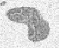
In the 16885 dataset, go to slice 213 and find the dark region
below and to the left of the centre of the image, as shown at the right.
Click on
.
If lines already exist in this .tr3 file, a list of
them will appear as a menu, with
at the top of the list. If no lines exist yet, only the
button will appear. Click on it and then on
.
When the menu for specifying line attributes appears, click on
.
A prompt will
appear near the bottom of the window, asking for the name of the new
line to be added.
It is best to name lines systematically.
For this exercise, name the line test1_213 (because the line
appears first in slice 213).
For this exercise you should use the
button to change the line from open to closed.
The can be left at its default value of zero for now. It will be considered later in the part of the tutorial dealing with finite-element simulation.
Click on to continue. Later you can change these attributes, or set other attributes, by doing .
There are three different methods available for
adding the points that define a line: manual, autotrace and flood.
The manual method is the most straightforward but also the most tedious.
The autotrace and flood methods can greatly speed things up – when
they’re successful. They work best for structures with good contrast.
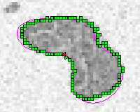
To add points to a new line manually, simply left-click in the image window. The prompt near the bottom of the screen will show the sequence number of the point to be added next. At any time the last point in the line can be deleted using the button.
Do not put points too close together. Doing so will make editing more difficult. In particular, do not attempt to connect lines by putting points on top of one another; the connection should be made using the start-at and finish-at features. Also, do not put the start and end points of a closed line on top of one another; the connection between them is made by declaring that the line is Closed.
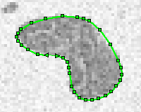
The image on the right shows a typical manually added closed line. Note that the start point is shown as a triangle pointing to the right, the end point is shown as a triangle pointing to the left, and a thin green line connects them.
By convention, objects should be outlined counterclockwise
and holes should be outlined clockwise.
The function in the menu will attempt to trace a boundary automatically. It will use the current last point as its starting point; if no points have been added yet it will ask for a starting point. It will ask you to point to a point that lies in the direction in which it should go. It will then attempt to trace a boundary that has properties similar to the boundary defined by the two points that it has been given to start with. It will continue tracing until it hits the edge of the visible image or until it runs into itself. Often it will trace successfully for a while and then go off course. In that case the function can be used to delete all of the points following a point that you specify. You can then add some points manually and perhaps try autotracing again.
The image on the right shows the result of autotracing this region with one manually selected starting point and selection of the direction in which to start. In this particular case it worked quite well.
Autotracing generally produces more points than you need,
and the result almost certainly needs to be
cleaned up.
The function in the menu traces a line around a closed region based on a range of pixel intensities. This method cannot be combined with the manual and autotrace methods.
Specify a location and a range of pixel intensities by defining a seed rectangle: point to two diagonally opposite corners inside the region you want to segment. Fie will attempt to trace a line around the desired region, displaying the result with small green symbols.
If the line isn’t quite right (or is terribly wrong), you can use the menu to adjust the thresholds.
Click on
when the line is satisfactory (or as satisfactory as it’s going to get).
If the line is mostly acceptable but part is not, the
function in the
menu
can be used to remove that part by pointing to each end of it.
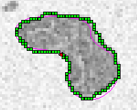
The image on the right shows the result of flood-filling this
region.
As with autotracing, flood fill
generally produces more points than you need,
and the result almost certainly needs to be
cleaned up.
Go to slice 214,
do and select The thin orange line that you see in edit-lines mode
represents the contour that you segmented in slice 213. If you
go back to slice 213, you’ll see a thin magenta line representing
the contour segmented in slice 214. You can
change the colours that are used for
displaying the lines in the previous and next slices.
When a line has been satisfactorily traced in one image, it is often
useful to immediately use the
button to advance to another image, rather than doing
. This way a line
can be added to multiple slices without having to specify the line
name each time.
The flood method works particularly effectively this way because
it automatically attempts to use the same location and intensity range
for the next slice.
Often you will not need to segment structures in every slice. If,
for example, every
fifth slice is enough to provide the desired amount of detail, then
it is convenient to set the ‘big step’
setting to 5 and then use the
to move from slice to slice.
When a line is segmented in multiple slices, the starting points should
be consistently positioned from slice to slice, because when Tr3
creates triangles between slices it always starts by connecting
the starting points. If you always use flood fill,
the starting points will generally be well aligned automatically.
If you use manual tracing or
autotracing, you need to make sure that you position the starting points
consistently. If the starting points are not well aligned, the
triangulation produced by Tr3 will be of poor quality.
The starting points can be changed later using
.
For the purposes of this tutorial, once you’ve segmented the structure
in two slices you’re ready to save your work and create a model.
As soon as you have done any work that is worth saving, go to the
main Fie menu and do . Each time you save, you will be asked to type in a comment
about what you’ve done. Entering a few words here may help in
recovering from problems later. The first time you save, you will also
be asked to type in your initials, which will be saved along with your
comments.
To create a 3-D surface model from the line(s) that you have created
in two or more slices, save your work in Fie and then
use the Tr3 programme. You do not need to exit
from Fie before running Tr3. Initially you can ignore all of the options
that Tr3 offers,
including the function,
and don’t worry about the message saying
Once Tr3 has created a Read the usage instructions for Thrup’ny to become
familiar with its features. When trying to understand what’s wrong
with a model, removing individual structures is useful for isolating
problems.
See Viewing and pointing
and Edit in the Thrup’ny documentation.
Switching the camera type to
orthographic is also often helpful.
Wireframe mode can be useful for detecting badly shaped
triangles.
If you’re using Fie within VirtualBox on a Windows host,
it’s probably better to install and use Thrup’ny
in Windows directly.
Thrup’ny is not available for Mac OS, so if your host is a Mac
you’ll have to use Thrup’ny under Linux.
If you’re using Thrup’ny under
Debian 10 (and possibly other versions of Linux),
you may need to try a few times before
Thrup’ny can successfully display a model. It is known to work well
under Debian 9 and Ubuntu 18.04.
An alternative to Thrup’ny is
Thrwp’ny, a Web-based viewer. To produce model files
for viewing in Thrwp’ny, select the
option in Tr3
and then either
(probably what you want) or
.
You must have already created a subdirectory called In the rest of the tutorial, whenever you try something new you should
save your work,
run Tr3, and use Thrup’ny or Thrwp’ny
to see the results of what you’ve done.
Once a line has been added, it can be manually edited
using the various tools of the
function in the main Draw menu.
Note that the Undo facility is extremely primitive. It can only be used
to undo the positioning of a single point, and only if undone immediately.
The best protection against errors is to save frequently.
The Autotrace and Flood methods often produce excessive numbers of points
and very jagged lines. The
and
functions can be used to clean things up somewhat.
The more powerful Snake function can also
be used for this (see When using the Manual method, it is sometimes useful to manually
specify only a small number of points and then use the
or
function to interpolate additional points.
An existing line can also be refined using the semi-automatic line-fitting
functions. The snake method is especially useful.
There are several ways of taking advantage of it:
Invoke the snake method by doing
then
then
.
Choose the line to be fitted from the menu that appears. A menu then
appears that offers a number of settings that can be adjusted.
See the detailed documentation for how to use the various adjustments.
The actual fitting is done by using the
the
button.
If the results of that slithering are bad, use either
or
to back up and try again.
If the snake algorithm is having trouble getting part of the line to
fit the desired boundary,
then
can be used to help it along. The functions are similar to those
for manually editing lines.
Once you are satisfied with the fit, or have given up, click on
. In the menu that then
appears, you can choose to keep the results of the fitting and go
directly to another slice. This allows efficient fitting of the same
line in a number of slices after having added it using, say, the flood
method. If the line that you were fitting does not already appear in
the new slice, the line will be pasted into the new slice, ready for
fitting. This allows efficient addition of a line to a number of
slices without having to do an explicit
for each slice. Whether it’s better to do a series of floods followed
by a series of snakes, or just do a series of snakes, depends on the
nature of the data and on personal preference.
When fitting an open (as opposed to closed) line in a sequence of
images, it is often useful to do a manual adjustment of the
first and last points before slithering
in each new image. When you click on
the first point in the line will be the active point. You can reposition
it by right-clicking, then use
to move
to the last point in the line and reposition it. Then click on
and try slithering.
When a closed line is triangulated in Tr3, a hole will be left at the
first slice and at the last slice. To close the hole you can use a
cap. Add a cap in slice 213
for the line that you have added in slices 213 and 214.
To add a cap, do and select . In the
menu that pops up, click on
.
In the next menu that pops
up, click on then select the line
that you want to cap, either by clicking on it in the image window or by
selecting it from the list of lines that appears.
Click on . The top-most menu will now display
the name of the selected line where it used to say
‘(undefined line)’. Select .
By default the cap will be put at the ‘head’ of the structure,
that is, at the first slice in which the line appears.
Fie will jump to that slice if it is not already there.
You can put the
cap at the last slice in which the line appears
by selecting and
then selecting .
Fie will then jump to the last slice.
Notice the message at the bottom of the window that says
. The cap must be given a name for it
to become active. Select
and type in a name. If you just type
a name will be assigned automatically, which
is usually the best option.
This should be done after specifying whether the cap will be at the head
or tail because the automatic name will
include either ‘_head’ or ‘_tail’.
Caps (and also joins) inherit attributes from the lines
that make them up so normally you don’t need to specify their colours,
material properties, etc.
In addition to specifying that a cap is
a head cap or a tail cap,
it is also possible to specify that the cap should appear
at the current z value
(i.e., in the current slice) or at some particular z value
entered using the keyboard.
However, these features are seldom necessary.
By default, Tr3 generates triangles
only between lines with the same name.
If, for example,
a structure is defined by a single line in some slices but by two
lines in other slices,
then the lines will need to have different names,
and therefore Tr3 by default will not generate triangles to join them
together. To tell Tr3 to do so, you must define a
join between the last slice in which the structure
has one configuration and the first slice
in which it has a different configuration.
(This implies that, in the Join definition,
the first line of the join should be in a lower-numbered slice
than the second line.)
In the 16885 dataset, go to slice 215. The structure that you have
segmented in slices 213 and 214 has almost split into two separate
regions, as shown at the right.
Add line In slice 216, add lines
Position yourself to view slice 215 and then
do . Select .
You will see that lines from two different slices are displayed:
those from slice 215 in dark green and those from slice 216
in dark magenta. The
menu that pops up has three sections. The first section consists
of buttons for and
. The other two sections are
separated by a dummy button labelled
.
Each of the two sections has a button
and a list of lines that initially just has one entry, labelled
. There is also a button
for specifying the z values of the slices involved in the join;
to begin with you can ignore this.
To define a line that’s involved in the first part of the join
(slice 215),
select . In the menu that
pops up, select and then
select the desired line ( As shown at the right,
the auxiliary windows under the main view show alternate representations
of the join definition. On the left is the single segment of the
first slice of the join. On the right are the two segments of the
second slice of the join. Red numbers correspond to the different segments
in each slice,
and black squares indicate the start of each segment.
Red half-arrowheads indicate the directions in which the lines
are traversed.
If we leave the join definition as it is, then Tr3 will connect
the first point of the line in the first slice
to the first point of the first line in the second slice,
and in the second slice
Tr3 will continue from the last point of the first line
to the first point of the second line.
In general, and in the example shown here, these different
starting points will not work well together and something
needs to be changed.
This could be done by using
to change
the lines’ actual starting points. However, this will often have
undesirable effects elsewhere. A better way is to modify the
join definition itself, which is what we’ll do here.
In our example, we’ll use the starting point of the
line in the first slice as it is but make changes in
the second slice.
(This is not the only possible approach.)
First, select the first line
in the second part of the join menu
(i.e., the button that says The next step is to
specify the for the line
by selecting the button . You can
again explicitly select a point. However, if you want Tr3 to trace
all the way around the line and back to where it started, which is what
is needed here, select
the button.
(If you specify the same point as where you started, it will just
stop there and not trace around the curve at all.
Using will specify a position just
slightly before the first point, causing it to trace all the way around.
You don’t need to specify for a closed
line that is starting at its actual start, because its default
start and end positions of 0 and 1 will automatically cause it to
wrap completely around.)
The buttons
and now display values between 0 and 1 that
correspond to fractions of the distance from the start of the line
to the end of the line, unless is used
for the end position. When is used,
a value of −1 will be displayed as a flag.
The next step is to specify that Tr3 should jump from line
The join is not quite finished; if you generate a model
now, you’ll see a triangular gap in the surface, as shown at the right.
In order to close the loop
in the second slice, it is necessary to jump from the end of the second line
back to the start of the first line.
Use the
button and add the first line again. Then select its menu entry and
use buttons and to
set both the start and end positions of this third instance of the line
to the start position of the first instance of the line, by selecting
the point highlighted by 3-pointed stars.
The complete join definition should look something like the menu
at the right.
The auxiliary windows should show something like the image at the right,
with three segments in the second slice of the join.
(The green lines don’t appear in the actual Fie display –
they’ve been added here to
emphasize that the topologies of the lines in the
two slices are the same, which is essential for a join to be correct.)
The diagram indicates
that Tr3 will start by connecting positions in the first and second slices
that are reasonably close together. Then, as it traces counterclockwise
around the line in the first slice,
it will first trace in the same direction around line 1 in the second slice;
jump to line 2 and trace around it; and then jump back to the original
starting position on line 1.
Similar to what you saw for your caps,
there is a message at the bottom of the window that says
. The join must be given a name for it
to become active. Select
and type in a name. If you just type
a name will be assigned automatically, which
is usually the best option. The automatic name will be the name of
the first line in the second part of the join.
The final join should look something like the image at the right.
(You can click on the image to view the VRML file.)
To make it easier to debug problems with joins, you can use the
button in the join menu to specify
a distinctive colour in which the join will appear in the 3-D model
created by Tr3. When you want to set the colour back to its default
value, select in that menu.
Important things to remember about joins:
To reiterate why joins are necessary:
by default, Tr3 generates triangles only between lines with the same name,
and sometimes lines must have different names in different slices even
if the lines belong to the same structure.
For example:
This section can be skipped on a first pass through the tutorial.
If a line changes shape dramatically from one slice to the next,
Tr3 may create long thin triangles between the two slices.
This is undesirable in a finite-element model.
To avoid this, you can use a different line
name when the shape changes and then use a combination of a join and a cap
to connect the lines.
The figure at the right illustrates a simple join (green)
between two such lines. The shape is the same as would be obtained by
just using the same line name for all four slices, and involves
long thin triangles where the shape changes a lot at the right.
The second figure on the right shows the use of a cap (magenta)
together with the join.
This section is important if you want to learn how to
run finite-element simulations
with a model. Parts of it
are also useful if you want to learn
how to prepare a model for 3-D printing. Otherwise just skip this section.
(For the purposes of 3-D printing, you can ignore the stuff
about material properties,
mesh resolution, thickness, boundary conditions and pressure, and when
using Fad you don’t need
to either run Gmsh or run Fad the second time.)
Starting from the lines created above, add the
line Make sure you have a head cap (but not a tail cap)
for Add material properties by doing
.
Select and use the menu to
specify the desired properties
(e.g., Young’s modulus = 20.M, Poisson’s ratio = 0.3,
mass density = 1000.) and a descriptive text.
Be sure not to include a space character between
Edit the attributes
for the three lines, setting
the
To be able to run a simulation, we need to define physically
reasonable boundary conditions. For example, in this model we can clamp
one of the small caps.
Edit the attributes of cap
To run a simulation, we also need to define a physically
reasonable load. For example,
we can apply a pressure to the unclamped cap.
Edit the attributes of cap Save the Run
FEBio
on the If the simulation runs for some number of time steps
then stops with
a negative-Jacobian error, it may be because your model’s
deformations have become too large; try reducing the pressure value.
If you’ve used the recommended material properties and this happens,
it may be because your model has badly shaped elements
or excessive roughness that cause
problems when the model is deformed.
Such problems should be addressed by revising
your segmentation, your lines’ starting points,
your join definitions, etc.
If you try to correct the model definition outside of Fie and Tr3,
you won’t later be able to go back and revise or
extend your segmentation using Fie.
The ultimate output in PostView
should be something like the figure at the right.
In the next few sections you will see how to use
open lines to create a
shared surface between two structures.
The ligament actually extends from slice 249
to about slice 264. We shall concentrate here on slices 254 to 261
for simplicity.
Go to slice 254 and find the part of the image shown
at the right. Create a closed line with the starting point at the
top, as shown in the figure.
Call the line
(In a case like this, no automatic method is going to work so you’ll have
to segment manually.
We start the line at the top because later we might
want to split the line further in order to model the joint between
the incus and the malleus, one of the other small middle-ear bones.)
To permit the creation of an explicit shared surface between
the bone and the ligament, you can now split the single closed line
Step 1: To first split the closed line into two parts,
do
.
Select For part 1, click on
and create a new line called
For part 2, create another
new open line called The result should look something like the figure on the right,
with two open lines.
Step 2: To create a third line, for the ligament,
use again to split
The result should look something like the figure on the right.
If you want to see what your model looks like so far, you may want
to skip forward to the section on subsets
before returning to the section below on connecting open lines.
The three open lines created in the previous section need to be
connected together in order to recover a closed boundary for the incus.
This is done by using the
start-at and finish-at
features in Fie.
You should never try to connect lines just by superimposing their points
or making them very close together. That approach won’t work at all for
making finite-element models or for 3-D printing, and it will also
make editing in Fie confusing and difficult.
To start, do
and select line Similarly, specify that Sometimes a line will need to start or finish on one line in
some slices but on a different line in some other slices. This is controlled
using the first four menu items.
We now want to add some open lines to represent
the posterior incudal ligament and its connection to the cavity wall.
In slice 254, the segmentation
should look something like the figure at the right.
The white lines
correspond to the medial and lateral surfaces of the ligament and could
be named The lower beige
line corresponds to the part of the wall of the air-filled middle-ear cavity
where the posterior incudal ligament is attached,
and could be named It is probably easiest to manually segment one line at a time from
slice 254 to slice 261
using and stepping
from slice to slice.
Segment the lines in the same slices in which
you segmented line As above, the different open lines need to be connected together.
In our example, the ligament lines are specified as starting
and finishing at the starts and finishes of the incus and cavity-wall lines.
One could equally well decide to have the cavity-wall line, for example,
start and finish at the ends of the ligament lines.
It is recommended that
lines be specified to start at a start or finish
which doesn’t itself depend on some other line
(as shown in the ‘Good’ panel, where lines A and B
both start at the finish of line C).
If line A starts at, say, the start of line B, but line B
itself starts at the finish of line C, then line A will not
start at the start of line C but rather at the first
‘real’ point of line B, as shown in the
‘Bad’ panel in the figure at the right.
If you want to create a 3-D model of the ligament, you need to
create caps at the top and bottom slices.
In this case, each cap definition will consist
of several lines.
The lines are combined together in a manner similar
to how the two lines were combined for the second slice of the join
above.
The individual lines must be listed in the order
in which they will be traversed to form the boundary of the cap.
The figure on the right shows the definition for a
cap for the ligament.
Note that the lines corresponding to the incus and the cavity
wall both have a minus sign in front of the line name. This is because
they must be traversed backward when being used for the ligament boundary.
The line corresponding to the incus would of course be traversed
forward when creating a cap for the incus.
A good practice is for the names of shared lines to include indications
of both structures that they belong to, with the one that their
direction corresponds to coming first. For example, the name
Backward traversal of a line is invoked by clicking
on item 1 in the manu that pops up when a line is added to the cap.
This changes the plus sign to a minus sign.
You will be asked if you also want to swap the start and end positions.
In most cases you should select , so the
line will be traversed backward from its end ()
to its start (;
see for more details.
The figure on the left shows what the menu looks like when specifying
line If you want Tr3 to create a model that contains only certain lines, you
can create a subset.
Do ,
select , and give the new subset a name.
In the menu that appears, select
to add a line to the subset definition and then enter the desired
text. In the simplest case, such a line will consist of a line name,
a colon and a space, and the text In the subset definition you can also override line attributes
like colour, transparency, etc., using
the attribute syntax. For example, if you wish
to generate a finite-element model,
but material types and thicknesses have not been specified as attributes
of the lines involved, they can
be added in the subset definition, as shown in the figure on the
right.
For this ligament subset, when creating a finite-element model
it is necessary to correct for the fact that the incus and cavity-wall lines
are backward, as mentioned in the previous section. This can be done by
adding If caps or joins form parts of shared surfaces, they also can be reversed
when necessary using The interactions between reversals of lines and of caps and
joins, and between reversals defined in subsets and those defined in
line, cap and join definitions, can be confusing. When in doubt, check
for reversals in Fad using To also change
the colour and x-y mesh resolution
for all of the lines in the subset,
the following line could be added: Once you have defined one or more subsets,
Caps and joins will automatically be generated by Tr3
for a subset if all of the
lines they require are included in the subset definition;
the caps and joins don’t need
to be explicitly included in the subset definition.
Sometimes a
line is needed in one slice for a cap or a join, but simply adding that
line to the subset definition would result in the unwanted creation of
the corresponding surface in the model by Tr3. A solution is to use the
To do a finite-element simulation of a system that includes
volume meshes for more than one structure:
This is an example of a place where a join is
required when a hole appears in a structure.
The figure on the right shows the lines involved at
the beginning of a hole in a structure, as displayed while defining a
join.
The green line and vector indicate a counterclockwise loop
with a deep indentation,
before the hole has closed. The magenta lines and vectors represent lines
in the next slice,
after the hole has closed. The magenta line forming the hole itself (item 2 in
the figure) has been traced clockwise, while the line around the outside
(items 1 and 3) has been traced counterclockwise.
In the second part of the join (magenta),
If you have already segmented a line with the same name
(say If you want to change the name of a line in all the slices in which
it appears, just use
to change its name attribute.
If you see a thin line with no points in slices where you don’t expect
it
(or an unexpected surface in your model),
reread the section on Applying the line-smoothing operation
()
to a manually
traced or edited line can make the line nice and smooth in each slice,
but it may make the resulting 3-D surface less smooth from slice to
slice, because the smoothing is done independently in each slice. The
operations can be used to produce
smooth surfaces but are best used after the surface is already
reasonably smooth, and the resulting lines should be carefully
compared with the corresponding images to make sure that they still
match.
Suppose you have revised a line and then realize that you want
to restore the line as it was in a previous version of your .tr3 file.
The following is one way to do so.
By default, Fie displays side views that display
lines that you have created. These side views are
particularly useful for seeing the range of slices that a line appears in,
and for checking the alignment of starting points.
You can control which lines are displayed.
You can also have side views that display orthogonal cuts through
the image stack. You can
toggle between the two modes using
.
Another way of seeing images as side views is to use the
Mark voxels feature.
If your triangulated surface looks strange,
use Thrup’ny or Thrwp’ny
to identify which lines, joins or caps are causing
the problems, and then use the
Verify option in Tr3 to see
what’s happening.
The Verify option can also be used to correct
certain kinds of problems using the
and
tools.
Having too many vertices and triangles in your model
will make the mesh difficult to debug;
may make model viewing slow;
may cause problems in Gmsh or at least make it very slow; and
will make finite-element simulations very slow.
If you have too many points in your Fie
segmentation, you can reduce the number by
using with appropriate settings,
or by specifying the
desired node spacing to be > 1 when using
snake fitting.
Alternatively, you can set the x-y mesh resolution to
a value that gives a reasonable number of triangles in your model.
This can be specified line by line, or it can be specified for
multiple lines in a subset definition.
If you get a message from Tr3 that there are too many nodes,
the maximum number is very generous,
so you really do have too many, especially for finite-element analysis.
Structures like blood vessels and nerves can often be conveniently modelled
using the tubing line type. Typically
the structure will be represented in each slice by just two points, defining
the centre and the radius. Tubing-type lines are very easy to smooth across
slices by using Smooth points across slices
for the (which defines the centre of the tube)
and for .
The following summarizes the functionality of Fie, organised
according to the items on the top-level menu (shown at right).
includes file opening, saving, etc.
includes a number of settings. Other than font size, the important
ones for most current uses are included at various places under .
allows the specification of focus
regions for operations like filtering and statistics.
includes various image-processing
operations.
provides a number of image filters.
provides some simple pixel-painting operations.
provides a sophisticated set of drawing and segmentation operations.
provides various kinds of statistics for pixels and clusters of pixels.
provides a number of image operations
like resizing, reshaping, distortion removal and alignment.
produces a combination image by combining
selected images from a stack of images, using either average or maximum
pixel values.
generates a 3-D surface from a stack
of images using a user-specified threshold and a marching-tetrahedra
algorithm. The surface is output as a VRML file.
just quits, after checking for any
unsaved modifications, and with saving of session settings.
Note that all of the
contour-tracing things are located under
, and the alignment tools for stacks of
histological images are under .
Fie can read in several different types of files, as described in
the following subsections. When Currently (for historical reasons) Fie handles JPEG images
differently from the way it handles other types of images. JPEG images
can be handled only by opening a
For new datasets that we create ourselves, the format of choice
is JPEG. It provides greater image compression and more flexibility.
Fie can read both grey-scale and colour JPEG images.
A 3-D stack consists of a set of image files, one image
for each slice.
The images in a stack must
all have the same numbers of rows and columns of pixels.
The usual practice is to have all of the image files
in a subdirectory of the directory where the Fie can read several types of TIFF-encoded images: 8-bit grey-level
or paletted, and 24-bit RGB, either uncompressed or with
run-length-encoding compression.
A 3-D stack of TIFF-encoded images must be stored in a single
multi-image TIFF file. The images must all have the same numbers of
rows and columns of pixels, and must all be of the same type.
If the file
Fie can read images, or stacks of images, stored as raw byte streams.
If the file
Any line which starts with a semicolon is interpreted as a comment.
Example. A stack of 8-bit grey images might have this
If no
Fie
will also look for a file These are grey-level files as used in
VolPack.
The
If the file
Fie can generate test images or new
Fie can generate test images and image stacks
with user-specified size and
various contents:
Fie can generate a new If you specify the same file for the first and last image, Fie will
reuse the same file for every slice, and will
ask how many such slices you want.
Fie will then ask for the file path and name to use for the new
Fie will then ask for the z coördinate to use for the
first slice, and for the z spacing between slices. It will
then ask for the x-y pixel size, which should be
measured in the same units as the z coördinates.
If you don’t know the actual dimensions at this point, you can
just accept the defaults and then adjust things later.
Finally, Fie will ask for your initials and a line of comment, and
create the new Fie can import surface definitions. An appropriate image stack
must already be available, and the stack should be opened before
doing the import. One way of preparing the image stack is to create
an initial
Fie can import contours traced by SurfDriver. The contours
must first have been Exported from SurfDriver to To export a set of contours from SurfDriver:
To import the contours, first use
to open the image stack. Then
do . You will then be asked for
Fie can import
Fie can save data in various formats:
See the descriptions in the
When using Fie to do image segmentation, the only file that needs
to be saved is the Saving a stack of images is a convenient way of converting the
images to a different format, e.g., converting a TIFF or raw image
stack to a set of JPEG images. When a stack of images is saved, they
will not include any changes made to them within Fie.
Same as Zoom
function within .
Same as Pan
function within .
Same as New image
function within .
Choose from several palette options.
For grey-scale images, the palette controls how the grey levels are
displayed, possibly with colour. Normally one would choose either
a grey-level palette (possibly specifying a gamma and thresholds) or
a false-colour palette.
For full-colour (3 bytes/pixel, RGB) images, the grey-level mapping
defined by the palette is applied to any pixel which is a shade
of grey, i.e., for which the red, green and blue values are the same.
This may be appropriate for images which are essentially grey-scale
but have annotations in colour.
For paletted images (1 byte/pixel colour) the selected palette controls
the mapping from the single-byte pixel value to colour.
Currently this applies only to TIFF images which are paletted;
such an image will set up its palette when it is read in.
allows adjustment of the pixel value below
which all values are displayed as completely black. By default the
black level is 0.
allows adjustment of the pixel value above
which all values are displayed as completely white. By default the
white level is 255 (i.e., the maximum pixel value).
and
correspond to two thresholds.
Pixels are set to shades of
blue if their values are less than the
first threshold, and to shades of yellow if their
grey-level values are greater than the second threshold.
Such thresholds can be used to assist segmentation.
The sample image shown here has the thresholds set to
differentiate among bone, soft tissue and no tissue.
As here, the distinction will generally be only approximate
and in itself cannot provide accurate segmentation.
False-colour palette ranging from black
through blue, green and yellow to white.
This palette provides
monotonically increasing brightness. It can be used
to enhance visual contrast and to make images prettier.
RGB encoded with 3, 3 and 2 bits, respectively
RGB encoded with ranges of 0 to 5, 6 and 5,
respectively
Palette starting with black and white; then
saturated red,
green, blue, cyan, magenta and yellow; then six
unsaturated colours having combinations of
0, 0.5 and 1 for r, g and b; then two greys;
then 30 shades each for grey, red, green, blue,
cyan, magenta, yellow and orange Black and white
Uses palette embedded in TIFF image (if any).
Pen size and shape for painting.
Partially broken and not used much these days.
The cursor shape for pointing can be either a crosshair (the default)
or an arrow. The cursor for text input has a T shape.
Specify whether certain operations are
to be applied to all of the image, to the visible part of the
image, or to specified focus regions.
Set size of main image window within the overall Fie window.
Click where you want the lower-left corner to be.
Sets or unsets watch mode for watching the progress
of certain operations.
Allows user to specify the name of a
command file for executing scripts (currently broken)
Sets the vertical size (an integer number of pixels)
of the overall Fie window.
By default Fie will guess at an appropriate window size, but sometimes
it will be too big or too small and will need to be set by trial
and error.
This setting is also used in
Tr3, Fad and
other Dip software.
Sets the font size (an integer) used in the interface.
This setting is also used in
Tr3, Fad and
other Dip software.
Specify various ‘focus’ regions, which can be used to
restrict the part(s) of the image involved in other operations
Apply various filtering operations
Things are painted into the image, actually changing the pixels.
This is here for historical reasons, and for playing with algorithms,
and isn’t really very useful at the moment.
Things are drawn over the image, not
actually changing the pixel values in the underlying image.
The x and y axes are the horizontal and
vertical axes, respectively, in the main image window,
with x increasing from left to right
and y increasing from bottom to top, as usual.
The z axis extends through the stack of slices
with z increasing from the first slice
to the last slice.
If the first slice is at the bottom
(e.g., the feet of an upright human body),
this results in a right-handed coördinate system;
if the first slice is at the top (e.g., the head)
it results in a left-handed coördinate system.
Most software used to process the output of Fie will
assume a right-handed coördinate system.
The
If images are displayed in the side views, the x-z
images are below the main image window and the
z-y images are to the left.
Left-clicking in such a sideview window causes the corresponding
slice number and z coördinate to be displayed.
Right-clicking in the window causes Fie to jump to
the slice corresponding to the z
coördinate where the click occurred.
Either left-clicking or right-clicking also causes either the
x-z image or the z-y image
to change to correspond to the x or y
coördinate where the click occurred.
If lines are displayed in the side views, they are in
two windows below the main x-y image window:
x-z
on the left and z-y on the right.
Left-clicking in such a sideview window
causes the corresponding z
coördinate to be displayed, along with the slice number and
corresponding z coördinate of the nearest slice.
Right-clicking in the window causes
Fie to jump to the
nearest slice that contains a line if that slice is reasonably
near by, otherwise it jumps to the slice nearest to the z
coördinate where the click occurred.
In the example on the right, all of the segmented lines are displayed
in the side views. If there are a lot of lines, this can make it difficult
to see individual lines. Which lines are included can be selected
using
a button in the menu.
The side views also include small tick marks indicating the
first and/or last nodes in each line, or even all nodes, as selected by
another button in the menu.
In Draw mode a scale bar
is displayed in the main image window. The units used for this scale
bar are specified in the
The first point
of a line is indicated by
a triangle pointing to the right
The image on the right shows how lines are displayed when being
edited. All lines in the current slice are green, except for the
currently active segment which is red. Lines in the previous and next slices
are shown as thin lines. The user can control whether all lines
in the previous and following slices are shown, or just the currently
active line, or none at all; and can control the colours used.
The rest of this section describes the various items in the Draw menu.
Zoom in or out by factors of two, or specify an integer zoom
factor. Zoom factors ≥ 1 correspond to magnifications. Negative
zoom factors ≤ −1 correspond to reductions; e.g., −2
corresponds to a magnification of ½.
As seen in the examples above, when zoomed in, the original pixels
are shown enlarged (rather than smoothly interpolated) so one doesn’t
lose sight of the resolution limitations of the data.
If the image is larger than the displayed area,
shift the display window by clicking in either the
overview window or the main image window, at the
point that you’d like to have centred in the display
window.
One can also recentre the displayed area by right-clicking
in either the overview window or in the main image window
when the main
menu is active, but not when the
menu is active.
(In mode, right-clicking
is used to reposition nodes.)
A 7-button navigation menu pops up, allowing selection of
a new image from the stack of images.
Set various parameters.
Many of the parameters
are saved in a session-settings file when
the user exits from the programme. The file is used to
restore the settings when the programme is run again.
When this menu item is selected, a new menu pops up listing the
subdirectories and containing a button for specifying a new
subdirectory. When a subdirectory is selected from that menu,
another menu pops up with options to modify the subdirectory name,
modify the image type, activate the subdirectory, or delete the
subdirectory from the list. (The subdirectory itself is not
affected.) The image type only needs to be specified if the
image-file names do not end with the file type (e.g.,
This button can be used to quickly toggle on or off the display
of lines in the main image window.
Copy lines to an internal clipboard
Paste lines from internal clipboard
Choose to edit a number of different things, including
caps, joins, labels, materials, attributes, etc.,
as shown in the menu on the right.
The first step in editing caps
is to select which cap to edit, or select
to create
a new cap. In the list of existing caps, if a cap’s name is preceded
by it means that the cap is defined
in an external file and cannot be edited
(except by opening the external .tr3 file).
For the next step, a cap-editing menu appears. The first two entries
are the usual Zoom and Pan operators, and the next entry is for editing
the attributes of the cap. The
item is for reversing the orientation of a cap definition, and is seldom
used. The item is for completely
deleting the definition of this cap.
Initially a cap definition includes a single
entry. Clicking on that button
brings up a line-editing menu, and the The first item of the line-editing menu initially contains a plus
sign (). Clicking on the button changes it to
a minus sign (), indicating that the line will
be traversed backward in forming the cap. The second menu item initially
says . Clicking on it brings
up a menu from which a line may be selected; a line may also be selected
by clicking on a line in the main image window. The button text then
displays the name of the selected line.
The last four buttons in the line-editing menu permit you to move
the line up or down in the list of lines making up the cap;
to delete the line from the cap definition; or to quit and
return to the cap-editing menu.
Buttons 3 and 4 initially say and
, respectively, and represent the fractional
positions along the line at which the part to be included in the cap
starts and finishes. Clicking on either button brings up a menu for
specifying the fractional position. Clicking on
or sets the fractional position to 0. or
1., respectively. Clicking on allows
the fraction (from 0 to 1) to be typed in. The most common method of
specifying a fractional position along a line is to select a point on the
line by clicking in the main image window or by using
the and buttons,
and then using the button.
The line name will be displayed in the cap-definition
menu with a minus sign in front if it is to be traversed backward,
and possibly with a start and/or end position in parentheses.
If the positions are (0.,1.) for a forward traversal, or
(1.,0.) for a backward traversal, the parentheses will not be displayed.
The editing of Joins
is not yet documented. It uses some of the same methods as editing caps.
See the tutorial for details.
The editing of labels
is not yet documented, but the menus should be fairly
self-explanatory if you understand the
syntax for labels.
The editing of springs
is not yet documented, but the menus should be fairly
self-explanatory if you understand the
syntax for springs.
The editing of concentrated loads
is not yet documented, but the menus should be fairly
self-explanatory if you understand the
syntax for concentrated loads.
The editing of Materials
is not yet documented.
Use this function to edit the attributes of either lines or slices.
You can choose to edit the attributes
of either a single line or multiple lines.
If you choose to edit the attributes for a single line, a menu
will appear which permits selection of one line.
After you select the line, a menu will appear in which each button displays the
current value of an attribute. Click on the appropriate button to
change an attribute. Clicking on
will allow you to select some other line from which all attributes
(except the name) will be copied to the line whose attributes are
being edited.
For some attributes (e.g., Open/Closed, Interpolation, Boundary conditions),
a menu will appear for selecting the new attribute
value.
For other attributes a simple text prompt will appear
asking for the new value.
If you choose to edit the attributes for multiple lines, a menu
will appear which permits selection of the lines to be affected.
After you select some lines, a menu will appear for editing only those
attributes which can sensibly be applied to multiple lines.
The attribute values will be preset to those for the first of the
selected lines. The only attributes whose values will be
transferred to the multiple lines are those whose menu buttons you use (whether
or not you actually change their values).
This attribute is set when the line is read in from either the main
Clicking on the button will switch
the Open/Closed attribute back and forth
between open and closed.
The button displays the current
line type.
Clicking on it brings up a menu for selecting the line type
that is desired. In some cases Fie can try to convert the existing
line data from the previous line type to the new one.
For the Colour attribute, a colour-selection tool will appear.
Find and click on the desired editing colour (the colour used within
Fie), then click outside the tool to make the selection. The
colour-selection tool will then appear again, this time for selecting
the rendering colour (the colour used for the 3-D models produced by
Tr3).
For the start-at and finish-at attributes,
each of the two menu
buttons displays the word
Clicking on button
offers a choice of ,
or .
(The option is dangerous
and should very seldom be used.)
By default the specification applies to all z’s, from
−∞ to +∞.
Clicking on button or
permits specification of a new z value.
You can either
Clicking on button
or toggles
between
The and buttons
move the current start-at or finish-at specification up or down in the
original list; the specifications
should be arranged in order of increasing z.
The button causes the current specification
to be deleted.
The two mesh-resolution menu items permit setting of the
x-y and z mesh resolutions.
Choose whether to edit the attributes for one slice at a time, or for
a range of slices: the current slice and all preceding ones, the current
slice and all following ones, or all slices. If one slice at a time,
the usual slice-choosing tool appears - use the tool to
position yourself to the desired slice and then click outside
the tool to make the selection. You will then be prompted for
new attribute values for the slice: z value, slice name,
rotation, and x and y offsets. The slice-choosing
tool then appears again; either select a new slice, or select the
same slice to quit.
If editing attributes for a range of slices,
the values requested are a z scale factor and a z shift.
The editing of subsets
is not yet documented. The actual lines of a subset definition
must be typed in, following the syntax
defined below.
When a new subset is created, it will automatically include the line
The editing of the names of ‘external files’
is not yet documented. External files are used when a set of images
is to be segmented by more than one person at a time.
Values for the x, y and z
scale factors for Tr3 files are requested one at
a time. By default, the y and z scale factors
will have the same value as the x scale factor.
This command causes Fie to jump to the slice and coördinates
corresponding
to the most recent Add a new line to an image or images. You are first asked to
either specify an existing line definition
or add a new one.
The line defining a particular structure should get a different
name (i.e., become a different line) when the boundary of the
structure changes its nature. For example:
If necessary, use to select a new image
from the stack of images. If a line has been
traced in the current image,
it will be saved before moving to the newly selected
image. Once at the new image, tracing can immediately
begin for a new line with the same name, unless such a line already
exists there.
Use and
as required.
The settings menu provides control over the smoothing algorithms used by
the function described below. The first three
buttons turn the three different kinds of smoothing on or off. The last three
buttons set the parameters for the different kinds of smoothing.
You can use the following functions to create the new line:
You are asked to specify two points
which define diagonally opposite corners of a
‘seed’ rectangle. The centre of
the rectangle is used as the initial seed point for a flood fill.
The range of grey levels within the rectangle determines which
pixels will be included within the flood fill, so the rectangle
should lie entirely within the desired region.
A boundary is traced
around the flood-filled region, with its starting point to the left
of the initial seed point.
A menu is then provided for
adjusting the thresholds:
For lines which are small and/or difficult, the line
is best specified manually point by point.
For long
stretches of clear boundaries, the autotrace function
works well. It continues until it runs into the edge of the visible
image, or until it runs into itself, or until it has generated
too many points. Usually it will go too far, and it may
also run off course. In either case
the trim function can be used to cut off the unwanted part,
and then the line tracing can be continued.
For closed regions with clear boundaries,
the flood function works well.
The manual and automatic tracing methods can be mixed
in any order, although the flood method is normally used
by itself, and will overwrite any previous tracing.
The median-filter and smooth operations
are particularly useful after the flood and autotrace functions,
which tend to produce jagged curves and many more points
than are required. The snake method of fitting
(
▶
▶
)
may also be useful after tracing here.
Edit the existing lines in this image.
Left-clicking within the image selects the closest point
to be the active point. Right-clicking within
the image repositions the currently active point.
Before using this function, first
position yourself at a slice in which you want
to do the splitting.
Also zoom and pan so that you’ll be able to see
the place where the split is to be made.
After then selecting this function, you will first
specify which line is to be split.
You will next specify which lines will correspond to parts 1 and 2
after the split. Often you will select for one or both lines. In that
case you will be presented with the menu for editing line attributes.
Change the line name and then click on . Notes:
You will next specify which slice or slices you want to do the splitting in,
by selecting a choice from a menu.
The actual splitting is done with a menu which allows you to select
the node where the split will be performed and then to associate that node
with one (or neither) of the two resulting line parts. Select the node
by using the
and
buttons
or by left-clicking on the node in the main image window, then press
,
or
.
If you have chosen to do the split in more than one slice, you will immediately
be moved to another slice, ready to select the node and do the split.
This continues until the requested slices have been processed. If at a
certain slice you can no longer see the place where the split is to be
made, press ,
do the required pan, and then restart the split operation. You’ll find
that the appropriate line-selection buttons have already been pressed.
You will first specify which line is to be snipped.
You will next specify which line will form the snipped-out part;
this will often be a new line.
You will then specify which line will form the remainder;
this may be the original line that is being snipped, or
it may be a new line.
The rest of the interaction for this function is similar
to that for the Split function. The part of the line to be
snipped out must not contain the original starting point
of the line being snipped. The line corresponding to the
remainder will consist of a concatenation of the parts
of the original line before and after the snipped-out part.
If the original line was a closed line, it may be necessary
to subsequently change the line corresponding to the remainder
to be an open line and to change its starting point.
Delete some or all of the lines in some or all slices.
Determine which slice(s) a line or lines
occur in. If a line has no points in any slice and
does not have both start-at and finish-at defined,
it can be marked for deletion even if it is
referenced by other lines or in definitions of caps, joins or springs.
Some functions repeated from
Apply scale factor and offset
An image stack is resliced perpendicular to the original plane of
section, and x-z and z-y views are
displayed. The side views are slices through a user-specified point.
The user can select that point by right-clicking in any of the
three image windows, or by using the menu.
Voxels can be ‘marked’, in which
case they will be displayed in a
distinctive colour.
Once you exit
from the Reslice mode the marked voxels can continue to be displayed
in the main image window. One use for this is to help with the segmentation
of structures which are difficult to visualise in the x-y
images. Another use of this feature is to mark particular voxels for display as
blocks in the VRML models produced by Tr3.
The remainder of this section explains the use of the menu.
Calculate density histograms
The model definitions created by Fie are stored in plain-text files with the
filename extension
A .tr3 file may contain the following sections:
*Whether section must be terminated by an
In the syntax specifications here, square brackets
( Within the The possible qualifiers are: The attributes are discussed in more detail below. All qualifier
names may be abbreviated to any unambiguous degree.
Most can
be abbreviated to a single character,
but, for example,
The circular cross-section of the tubing is represented by
a polygon in the generated model. The number of sides of
the polygon is controlled by
ires_xy.
In line definitions,
In subset records Start-at and finish-at specifications are used to connect
lines together precisely, without depending on superimposed points.
This is especially useful for creating closed surfaces using open lines.
You should not try to connect lines just by making their points
very close together.
For many purposes, including the 3-D surfaces created
by Tr3, a line will be considered to start
at its specified start-at point (if it has one),
not at its own first point, and
to finish at its specified finish-at point (if it has one).
Start-at and finish-at points work similarly; the description
below is just for start-at points for simplicity.
4.4.4 Doing multiple images
test1_213
from the list of lines,
and then trace the outline of the same structure.
You’re using the same line name, test1_213,
because Tr3’s default
action is to create a triangulated surface for a line that appears
with the same name in multiple slices.
4.5 Saving your work
4.6 Creating and viewing a 3-D model
No real elements, no .sap file created.
.wrl (VRML) file for your model,
use the Thrup’ny programme to view the file.
If you have used the default settings in Tr3, the file name of
the .wrl file will include _dbg (for
‘debug’ mode) and the labels that Thrup’ny displays
in pointing mode
will be the line, join and cap names that were used in Fie.
json
in the directory that your .tr3 file is in.
Point your Web browser at the .html that is created
in your json/ subdirectory.
If your model is not displayed,
see Using Thrwp’ny with local files for more information.
4.7 Editing a line
4.7.1 Manual editing
4.7.2 Cleaning up
Fitting a line below).
4.8 Fitting a line
4.9 Adding a cap
4.10 Adding a join
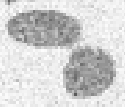
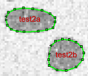
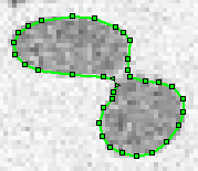
test1_213 in slice 215
using
with a
= 130 and = 80.
This should create a single line around the structure.
(As often happens, it is difficult to decide on the exact slice at which
a structure goes from being one region to two regions, or vice versa.)
Smooth the line.
test2a_216
and test2b_216 for the two separate regions.
They should again be Closed lines.
Also add the two lines, with the same names,
in slice 217.
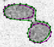
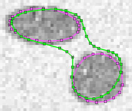
test1_213 in this case),
either by clicking in the image or by selecting
it from the list that appears. Similarly, to define a line that’s involved
in the second part of the join (slice 216),
select and specify the line.
To define the second line that’s involved in the second part of the
join, select the
button after the button
and then specify the line.
Because of the direction in which the lines are traversed,
this example will work better if you specify
line test2b_216 first and then
line test2a_216.
Note that the selected lines
are now displayed in light green and light magenta, and with larger symbols,
as in the image to the right.
(Click on the image to see a larger version.)
The starting and ending points to be used by Tr3 for
the join are indicated by
right-pointing and left-pointing 3-pointed stars.
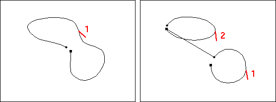
A bad join definition
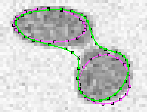
test2b_216)
and then select button
, which initially displays the value 0.
You are now prompted to specify the desired
for this line.
Select a point on this line which is reasonably close to the starting point
of the line in the first slice, and also close to points on the second
line in this slice.
Usually this
is done by clicking on a point in the image and using the
button.
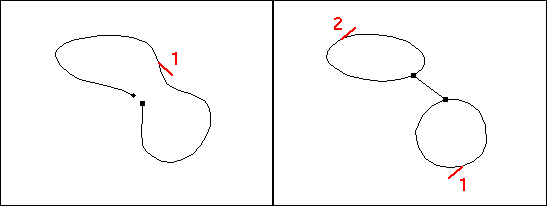
A better join definition
test2b_216 to line test2a_216. Do this
by clicking on the menu button that says test2a_216
and then select button . Select the point
that you want Tr3 to jump to as the starting position for this line.
Again specify that you want Tr3 to trace all the way around the line,
by selecting .
The result is as shown in the image at the right.
Note the display (for the magenta lines) of the newly defined
starting and ending points by superimposed left-pointing and right-pointing
3-pointed stars.
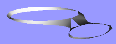
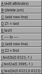
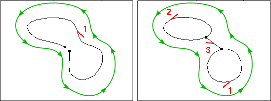
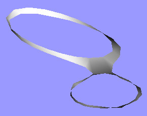
The lines should be
named systematically.
A,
and also in a later set of slices C,
but in intervening slices B it corresponds to only part
of the structure, then the line name must be different in both
B and C than it is in A.
4.11 Combining a join and a cap
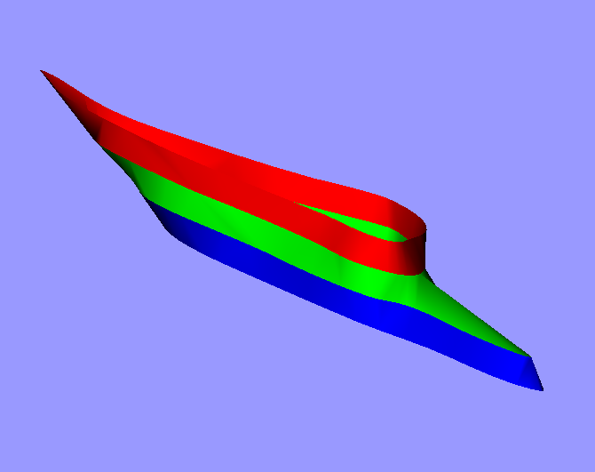
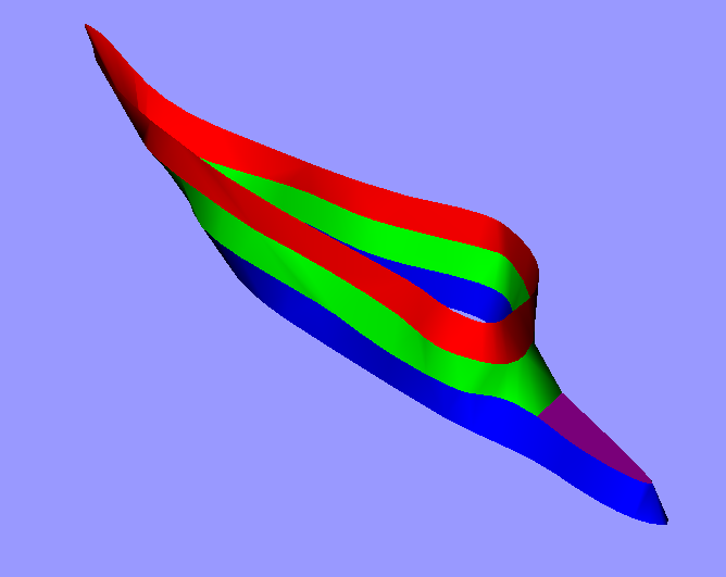
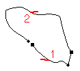 The figure on the left shows how
the join has been defined to include only part
of the blue line, by going from the beginning to about position 0.18
and then jumping to about position 0.43.
The cap fills in the rest of the space in that slice.
(This example is based on a structure in the lower left part
of slices 185, 190, 195 & 200.)
The figure on the left shows how
the join has been defined to include only part
of the blue line, by going from the beginning to about position 0.18
and then jumping to about position 0.43.
The cap fills in the rest of the space in that slice.
(This example is based on a structure in the lower left part
of slices 185, 190, 195 & 200.)
4.12 Creating a finite-element model
test1_213 in two earlier slices (211 and 212) and add the
lines test2a_216 and test2b_216 in two following
slices (217 and 218).
Line test1_213 should be renamed to
test1_211 to continue following the
recommended naming conventions;
this can be done using
.
test1_211 and tail caps (but not head caps)
for test2a_216 and test2b_216.
The units are not specified but will be assumed
by the finite-element solver to be consistent.
See
Units in FEBio.
The usual preferred choice is SI
MKS units.
If your mesh coördinates are specified in
mm or
um (μm),
for example, the units for other quantities must be adjusted
accordingly.
20. and M, as described in
Material properties.
x-y mesh resolution to 25;
the Material type to 1 (the one that you just defined); and
the Thickness to 1 (which is an arbitrary value that will
not be used.
You may need to specify a higher x-y mesh resolution if you have segmented
more than just the test lines.
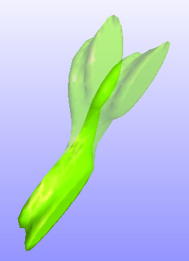
test2a_216_tail, setting
the Boundary condition to Clamped.
Clamping the cap itself only clamps the internal nodes of the cap.
You should probably also clamp the line(s) that form
the cap, especially if the cap is small.
test2b_216_tail, setting
the Pressure to 1 (another arbitrary and unused value).
.tr3 file and run Tr3.
If you’ve specified the material type and thickness, you should
get both a .wrl file and a .sap file.
Follow
the instructions for installing Fad
and then follow the
instructions for using Fad with Gmsh:
reading the .sap file;
checking it for correctness;
and using Gmsh to create a tetrahedral mesh.
At the end, export an FEBio file from Fad.
(Just type Enter in response to
the question about rigid elements.) Specify a pressure of
10k when asked.)
.feb file exported from Fad.
Make sure to use a recent version of FEBio.
4.13 Splitting to create open lines
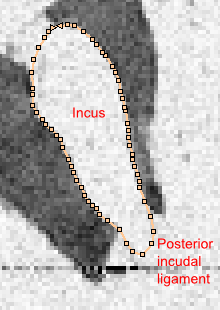
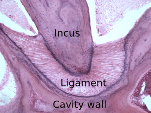 Between slices 250 and 261, the incus (one of the three
small bones in the middle ear) is connected to the posterior
incudal ligament,
which is connected in turn to the wall of the middle-ear
air cavity. The histological image on the left shows these structures
more clearly. The ligament is barely distinguishable from bone
in the MRM images.
Between slices 250 and 261, the incus (one of the three
small bones in the middle ear) is connected to the posterior
incudal ligament,
which is connected in turn to the wall of the middle-ear
air cavity. The histological image on the left shows these structures
more clearly. The ligament is barely distinguishable from bone
in the MRM images.
osinc_254, based on
‘os’ for bone, ‘inc’ for incus and slice number 254.
Create a similar line with the same name in slice 261 and in however
many lines you feel like in between.
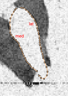
osinc_254 into three open lines. This needs to be done
in two steps.
osinc_254 as the line to be split.
osinc_med_254 (the medial side of the incus).
Use to
copy the attributes of osinc_254, then change
from closed to open.
Click on .
osinc_lat_254
(for the lateral side of the incus)
and again copy attributes and change the line
from closed to open.
In the next menu select .
You will now be presented one by one with the slices in which osinc_254
occurs. In each slice,
select the point on osinc_254
where you want to split it
(where the ligament surface
meets the bone on the left) and select
.
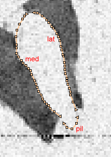
osinc_lat_254 into osinc_pil_254 (new)
and osinc_lat_254 (existing).
4.14 Connecting open lines
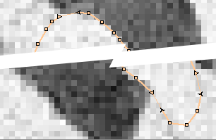
osinc_pil_254.
In the Attributes menu select
and then select . A new menu
item will appear – click on it
and a new menu will appear.
Menu button will contain the name of
some default line – click on the button, select
line osinc_med_254 and click on .
The triangle at the start of line osinc_pil_254 will
change shape and a thin line will appear connecting it to the finish
of line osinc_med_254.
osinc_pil_254 should finish at
the start of osinc_lat_254 and that osinc_lat_254
should finish at the start of osinc_med_254. The results
should look something like the figure on the right.
4.15 Creating structures with a shared surface
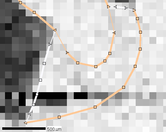
ligpilmed_254 and ligpillat_254.
Note that their orientations (top to bottom for the one on the left,
right to left for the one on the right) are appropriate for a
counterclockwise boundary for the ligament.
cav_pil_254.
Note that its orientation (top right to bottom left) corresponds
to a clockwise boundary for the cavity,
because it’s a hole and not an object.
osinc_254.
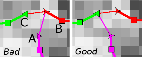
4.16 Creating caps with open lines
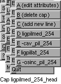
osinc_pil_254 has the incus first and then the ligament,
because the direction in which it was segmented
corresponds to its use in the incus.

cav_pil_254, for example, as part of the cap. Menu
item 1 contains a minus sign. Menu item 3 specifies that the traversal
of the line should start at the finish, and
menu item 4 specifies that the traversal should finish at the start.
4.17 Creating a 3-D model with a subset
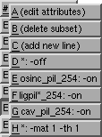
-on to specify that
the line is to be included
in the subset:
name:␣-on
where ␣ indicates a space character.
If lines are named systematically,
then wildcards can be used to make it easier
to define subsets. For example:
xxx*:␣-on
applies to any line whose name starts with xxx.
The figure on the right shows what the subset definition
would look like for the posterior incudal ligament.
-reverse (or just -rev) to the specifications
for the lines
osinc_pil_254 and cav_pil_254
in the subset definition.
(For -rev to have an effect,
-on must also be specified for the line in question.)
-rev,
by adding a line like
(cap)␣capname:␣-rev
or
(join)␣joinname:␣-rev
to the subset definition
(see Subsets).
p /fill and modify the model
definition using trial and error if necessary.
*:␣-c␣red␣-xyr␣150
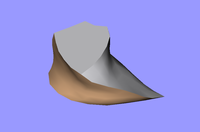 when you run Tr3 it will
display a list of the available subsets, and the name of the selected
subset will be included in the names of the model files created by Tr3.
The
animation on the right shows the model produced by the
when you run Tr3 it will
display a list of the available subsets, and the name of the selected
subset will be included in the names of the model files created by Tr3.
The
animation on the right shows the model produced by the pil
subset above.
do_slices line attribute
(together with -on)
to specify
that the line is to be included in the subset
only in the first or last slice
(or perhaps in both the first and last slice)
in which it appears.
(If do_slices both is used,
Tr3 will not create a triangulated surface for the line
even though the line is present in more than one slice.)
4.18 Creating a finite-element model from multiple subsets
.sap file for the
tetrahedral mesh for each structure.
r /sec command to read in the volume-mesh
.sap files for two structures.
j
with a threshold of zero.
Any shared surfaces among
the structures will be fully connected in the combined model.
w to
write out the resulting combination as a .sap file.
r)
if you need to read the .sap file for
the combined volume mesh back in.
When reading volume meshes, Fad reports on numbers of faces
rather than edges, and there is no need for any of them to be zero.
e)
to export the model as a finite-element file
(e.g., as an FEBio file).
4.19 Tips and tricks
4.19.1 Creating a join for a hole
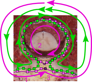
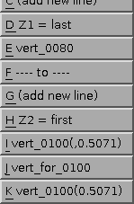
The figure on the left shows what the corresponding join definition might
look like, with segments 1, 2 and 3 defined by items ,
and .
The details would be different, of
course, if the starting points of the lines were in different locations.
4.19.2 Renaming a line in some slices
body2_020) across multiple slices and then realize
that you need to give the line different names in different slices, do
the following. Position yourself at the slice in which the
line body2_020 should start having a new name, and use
the command . When asked for
the , select the
line body2_020. When asked for the , select from the
menu and create a new line (similar to what you do when you add a new
line). Remember the
recommendation that each line name should
include the slice number in which that line first appears. Then, in
this case, select the menu item
.
4.19.3 Unexpected lines
start-at
specifications,
particularly the part about lines having both
-start and -finish specifications.
You may need to specify a z range.
4.19.4 Creating smooth surfaces
4.19.5 Restoring an old version of a line
lineToBeRestored.txt. Remove
the version number from the name of the previous version, so it becomes
the latest version again.
lineToBeRestored.txt in a text editor. Delete
everything up to and including the line that says DATA.
Then delete the END line at the end of the DATA
section and everything that follows. (That will include the
MARKED_VOXELS and COSTS sections.)
Save the file.
END
line at the end of the DATA section. Insert the contents
of lineToBeRestored.txt just before the END line.
Save the .tr3 file.
4.19.6 Side views
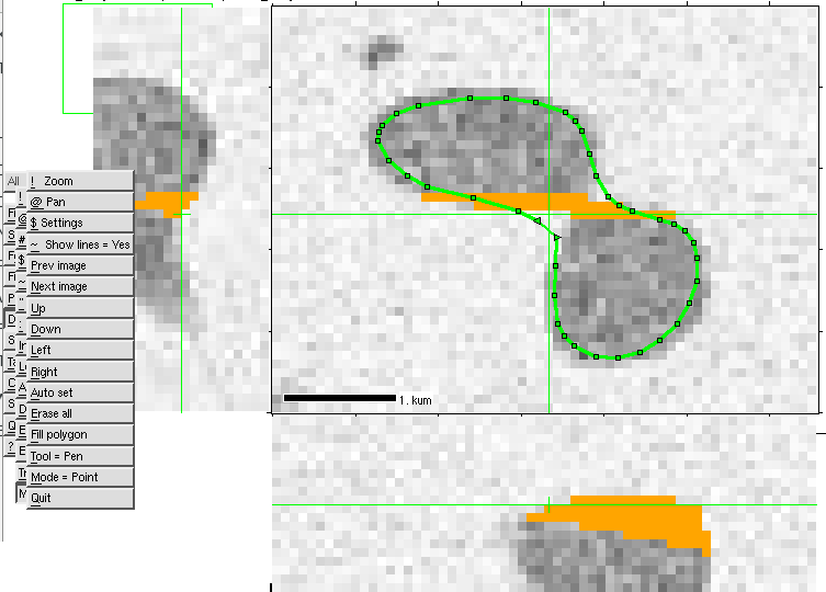
4.19.7 Triangulation problems
4.19.8 Too many vertices and triangles
4.19.9 Tubing

5. Menus
File
Set
Focus
Filter
Paint
Draw
Stats
Tailor
Combine
Surface
Quit
?
5.1 File
Open
New
Import
Save
5.1.1 Open
Open is selected from the
File menu, Fie will display a list of recently opened
files (if any). If the desired file appears on that list, select it.
If not (or if no such list is available) click on
or use the + shortcut key.
Fie will then display a list of the
subdirectories and files within some starting directory. (The
particular starting directory used may depend on which files have been
opened recently, on whether the HOME environment variable
is defined, and on the phase of the moon.)
Browse to find the file to
be opened and click on it.
.tr3 file which includes
a list of a set of JPEG images. For other types of images, open the
image file itself; Fie will then automatically open the corresponding
.tr3 file if it finds one with the same name as the image
file.
5.1.1.1 JPEG (
.jpg).tr3
file is. The name of that subdirectory, and the names of the
image files, are specified in the SLICES
section of the .tr3 file.
5.1.1.2 TIFF (
.tif)name.tif is opened, then Fie
will look for a file name.tr3 in the same
directory, and open it if found.
5.1.1.3 Raw byte stream (
.raw)name.raw is opened, then Fie
will look for a file name.fie in the same
directory. This is an auxiliary plain-text file which provides
the image size and other characteristics.
It contains lines with the following syntax:
NPIXH nh
nh = no. pixels horizontally
NPIXV nv
nv = no. pixels vertically
NSLICE ns
ns = no. slices in image stack
NBITS nb [nbu [{
SWAP|NOSWAP}]]nb = no. bits/pixel = 8 or 16. If nb=16, then nbu = no. bits actually
used/pixel = 8 or 16; and byte order is specified as either SWAP or NOSWAP.
Default no. bits/pixel = 8. If no. bits/pixel = 16, default no. bits
used/pixel = 16 and default byte order = NOSWAP.
TYPE t
t = image type: GREY or RGB.
Default = grey.
.fie file:
;15516.fie
NPIXH 228
NPIXV 186
NSLICE 168
NBITS 8
TYPE GREY
.fie file is found, Fie will query the user
for the image characteristics.
name.tr3 in the same
directory, and open it if found.
5.1.1.4 Density files (
.den).den file format includes a header which specifies, among
other things, the numbers of rows, columns and slices.
name.den is opened, then Fie
will look for a file name.tr3 in the same
directory, and open it if found.
5.1.2 New
Image
Tr3 file
.tr3 files.
5.1.2.1 Image
5.1.2.2 Tr3
.tr3 file corresponding to
an existing set of .jpg or .png files.
It will first ask
to confirm that you have such a set of files. If you answer
, it will ask you to select the
first file in the set, and then to select the last file in the
set. All of the image files
must be in the same directory.
Fie assumes that the filenames of every file in the set
consist of the same text followed by a sequence number (with leading zeros if
required), e.g., cat01.jpg, cat02.jpg,
… cat20.jpg. It asks what increment to
use for the sequence numbers; the default is 1, but you could
specify, e.g., 2 if you only wanted to use every second image,
or if you only had cat02.jpg, cat04.jpg, etc.
.tr3 file. It will offer a default path and name based on
the path and names of the image files.
.tr3 file. The file can now be opened
using .
5.1.3 Import
SurfDriver v. 2 (.txt)
SurfDriver v. 4 (.txt)
MRP
.tr3 file based on images corresponding
to the surface to be imported.
5.1.3.1 SurfDriver
.txt files,
and the corresponding set of image files used by SurfDriver must
have been used to create a .tr3 file.
.xdv file. If you get a message saying
Could not find slice file, click ,
browse to find the specified image file, and select it.
When the Slice Characteristics file appears,
click to accept it.
Get adjustment file window appears, browse
to find the .adj file and open it.
.txt
file and specify a name for it. The name should not contain
space characters; it is best to use only letters and numbers,
the hyphen and the underscore.
.xdv file to .txt,
repeat this process, answering when
asked Do you want to save changes to files?
You will then be asked to specify one or more .txt files. For
each file you will be asked to specify a short Prefix text string
to be used (combined with sequence numbers)
in forming the contour names in Fie. Once the contours have
been imported, you can use
to change their
attributes
from the defaults assigned by Import.
5.1.3.2 MRP
0 13502 27000
[landmarks]

[nodes]
2.0781 2.3786 1.9818
2.0789 2.3786 1.9924
2.0753 2.3647 1.
…
2.4724 2.9489 2.3444
2.468 2.9474 2.3474
2.4756 2.9458 2.3422

[surface]
1 2 3
1 3 4
5 6 7
5 7 8
…
.mrp files. This is a rather primitive
surface-definition file format; an extract from an example file is shown
on the right.
Landmarks are ignored. It is assumed that nodes come before triangles.
5.1.4 Save
Open section for more details
about some of the file formats.
.tr3 file. The images themselves are
not modified.
5.2 Set
! Zoom
@Pan
#New image
Palette
Pen
Cursor shape
Region of interest
Window size
Watch processing
Indirect input
Dip device size
Dip font size
5.2.1 Zoom
5.2.2 Pan
5.2.3 New image
5.2.4 Palette
Grey
False colour
3-3-2
5-6-5
RGB-CMY
B & w
TIFF
5.2.4.1 Grey
Black
White
Gamma
Blue
Yellow
Quit
[<
<<
<(
?
)>
>>
>]
 The grey-level palette controls the mapping of 8-bit pixel values
to displayed grey levels or colours.
A submenu and thumbwheel are provided for adjusting the black level,
white level, gamma, low (blue) threshold and high (yellow) threshold.
The default palette just maps
pixel values of 0-255 linearly to the same range of greys.
The grey-level palette controls the mapping of 8-bit pixel values
to displayed grey levels or colours.
A submenu and thumbwheel are provided for adjusting the black level,
white level, gamma, low (blue) threshold and high (yellow) threshold.
The default palette just maps
pixel values of 0-255 linearly to the same range of greys.
is the exponent of
a non-linear mapping from pixel value (v) to grey level (g):
g = vγ.
The default value of gamma (γ) is 1.0, corresponding
to a linear mapping.
Adjusting γ is sometimes useful to enhance contrast in
grey-scale images. These examples show the
grey-level palette with γ = 0.5 and 1.5.
γ=0.5
γ=1.5
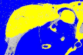
5.2.4.2 False colour
5.2.4.3 3-3-2
5.2.4.4 5-6-5
5.2.4.5 RGB-CMY
5.2.4.6 B & w
5.2.4.7 TIFF
5.2.5 Pen
5.2.6 Cursor shape
5.2.7 Region of interest
5.2.8 Window size
5.2.9 Watch processing
5.2.10 Indirect input
5.2.11 Dip device size
5.2.12 Dip font size
5.3 Focus
You can then specify how many rectangular focus regions
to generate with the specified symmetries, and the
parameter(s) used to generate them
5.4 Filter
5.5 Paint
5.6 Draw
5.6.1 Introduction
MIRROR option in a
subset definition can be used
to reverse the coördinate system.
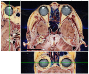
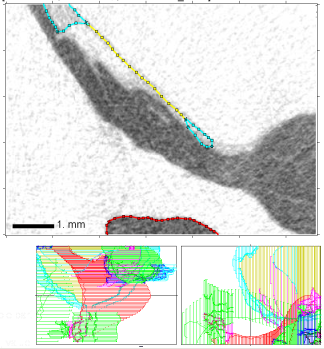 In addition to the main image window and the overview window,
two additional windows appear.
They are used for displaying side views of either the
stack of images (as shown on the left) or
the lines used to segment the images (as shown on the right).
Whether images or lines are shown can be controlled using
menu.
In addition to the main image window and the overview window,
two additional windows appear.
They are used for displaying side views of either the
stack of images (as shown on the left) or
the lines used to segment the images (as shown on the right).
Whether images or lines are shown can be controlled using
menu.
XY_CALC command.
 The image on the left shows how lines are displayed when not being edited.
Their colours, the line thickness and the symbol sizes can all be
controlled by the user.
The image on the left shows how lines are displayed when not being edited.
Their colours, the line thickness and the symbol sizes can all be
controlled by the user.
 and the last point of a line is indicated by a
triangle pointing to the left
and the last point of a line is indicated by a
triangle pointing to the left
 . First and last points
of lines which start at or
finish at the ends
of other lines are displayed as right-pointing
. First and last points
of lines which start at or
finish at the ends
of other lines are displayed as right-pointing
 and left-pointing
 3-pointed stars
(like dehydrated triangles).
Other points are shown
as squares. Connections due to
start-at/finish-at commands are shown
as thinner lines.
3-pointed stars
(like dehydrated triangles).
Other points are shown
as squares. Connections due to
start-at/finish-at commands are shown
as thinner lines.
5.6.2 Zoom image
In
Out
Specify
5.6.3 Pan image
@ Pan
5.6.4 New image
[<
<<
<(
?
)>
>>
>]
▶
# New image
5.6.5 Settings
Sideview: lines or Images
Sideview: which lines
Sideview: nodes = which
Next/previous slices: which lines
Next/previous slices: line Colours
Marked-voxel colours
Show marked voxels = yesNo
Pen size = size
Symbol size = size
Visibility of lines
Force visibility = yesNo
Image path = path
No. slices for big step = n
Grey-level mapping
RGB channel display
Window size
Autobackup frequency = n
-
which nodes are displayed in the side views.
, and
mean
that the first and/or last node in each line is joined
from slice to slice in the side view.
First
Last
First & last
All
Selected
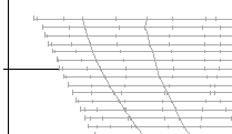 means that, in addition, small
tick marks are used to indicate the positions of all nodes;
this really clutters the display but it
may be useful in certain situations.
allows the user to specify
which node will be highlighted by joining it from slice to slice;
this is really only useful if a line has the same number of nodes
in every slice.
means that, in addition, small
tick marks are used to indicate the positions of all nodes;
this really clutters the display but it
may be useful in certain situations.
allows the user to specify
which node will be highlighted by joining it from slice to slice;
this is really only useful if a line has the same number of nodes
in every slice.
.jpg or .png).
-
set how many slices
are jumped when the and
buttons
are used to change slices. Default value is 10.
[<
<<
<(
?
)>
>>
>]
-
specify which colour channel(s) should be displayed.
Any combination of the red, green and blue channels can
be displayed;
or a difference channel (red–green,
green–blue or blue–red) can be displayed.
Red
Green
Blue
1 red minus green
2 green minus blue
3 blue minus red
*All
~Inv
5.6.6 Show lines
~ Show lines = Yes
5.6.7 Copy lines
5.6.8 Paste lines
5.6.9 Edit other
! Zoom
@ Pan
# New image
Edit caps
Edit joins
Edit labels
Edit springs
Edit concentrated loads
Edit materials
Edit attributes
Edit subsets
Edit external files
Edit scale factors for Tr3
Quit
5.6.9.1 Edit caps
! Zoom
@ Pan
A (edit attributes)
B (reverse cap)
C (delete cap)
D (add new line)
E (undefined line)
(undefined line) text
will ultimately be replaced by the name of a line (possibly with qualifiers).
The button is used for adding
another menu entry, which in turn
is used to bring up the line-editing menu.
1 +
2 (undefined line)
3 0.
4 1.
Up
Down
Delete
Quit
Prev
Next
Start
Finish
Keyboard
Select
Cancel
5.6.9.2 Edit joins
5.6.9.3 Edit labels
5.6.9.4 Edit springs
5.6.9.5 Edit concentrated loads
5.6.9.6 Edit materials
5.6.9.7 Edit attributes
Edit line attributes
Edit slice attributes
5.6.9.8 Edit line attributes
1 line
Multiple lines
External = yes_or_no
* Copy attributes from another line
Name = line_name
Description = descriptive_text
Open/Closed = open_or_closed
Interpolation = line_type
Colour = colour1;colour2
Transparency = 0_to_1
Shininess = 0_to_1
Start-at = independent_or_dependent
Finish-at = independent_or_dependent
X-Y mesh resolution = nel_per_diam
Z mesh resolution = n_slices
Material type = material_type
Boundary conditions = bc_code
Pressure = value
Thickness = value
/OK
5.6.9.8.1 External attribute
.tr3 file or an external file.
This attribute cannot be set directly in this menu, but it can be set
indirectly by using the
function.
5.6.9.8.2 Open/Closed attribute
5.6.9.8.3 Interpolation
5.6.9.8.4 Colour
5.6.9.8.5 Start-at and Finish-at attributes
1 -big
2 <
3 <=
4 5.
5 Finish of
6 wallextfr_001
Up
Down
Delete
Quit
Dependent if there are any such
conditions, and how many there are; or the word
Independent if there are none. Clicking on the button
causes a menu to be presented which displays the current start-at
or finish-at specifications, and a
button which can be used to create a new start-at or finish-at
specification with default settings. Clicking on the button for an
existing specification causes a menu to appear which displays
the current settings. For example, the menu shown on the right
corresponds to a connection to the finish-of
the line wallextfr_001.
±big
in the menus);
< and ≤.
In the example on the right, the first four buttons
indicate, for example, that the specification should be applied to the
range –∞ < z ≤ 5.
5.6.9.8.6 Mesh resolution
5.6.9.9 Edit slice attributes
5.6.9.10 Edit subsets
*: -off. That line should always be kept as the first line of the
subset definition.
5.6.9.11 Edit external files
5.6.9.12 Edit scale factors for Tr3 files
5.6.10 Jump to Fad location
Locate command
in Fad.
5.6.11 Add line
! Zoom
@ Pan
# New image
$ Settings
Flood
Autotrace
Delete last pt
Trim tail
Cut
Smooth
Quit
Median smoothing On
Average smoothing On
Spline smoothing On
1: Half-width for median smoothing = 1
2: Half-width for averaging = 2
3: Max. errors for spline smoothing = 0.2,0.25
-
traces a line around a closed region based on a range of
pixel intensities.
Lower threshold
Upper threshold
New seed
Quit
[<
<<
<(
?
)>
>>
>]
![[grey scale]](fie_draw_greyscale.png)
If the threshold adjustment goes too far and no filling can be
done, a warning message will be given;
use to re-initialise the seed
location and thresholds.
If a flood fill was done in a previous image for the same line,
then the last-used seed location and thresholds
from that image will
be used when is started
in a new image. If those settings aren’t able to produce a
successful fill in the new image, Fie will immediately ask for a new
seed location, defined by a single point, and will attempt
to use that seed location with the same thresholds that
were used in the previous image. This makes it easy to
re-use the same thresholds across many images, for
consistent segmentation.
5.6.12 Edit lines
! Zoom
@ Pan
# New image
$ Settings
~ Show lines = Yes
Snap to lines = No
Next pt
Prev pt
( Nudge left
) Nudge right
+ Nudge up
- Nudge down
Coords from keyboard
Delete pt
Cut
Insert pt
Append pt
Undo repositioning
Line ...
! Zoom
@ Pan
# New image
$ Settings
" Copy lines to clipboard
: Paste lines from clipboard
Locate line
Split line
Snip line
Concatenate lines
Shift boundary between lines
Rename line
Duplicate line
Reverse line
Orient line ccw or cw
Change start pt
Insert points
Fit line
Resample line
Xform line (scale/shift)
Smooth
Prev
Next
Point -> part 1
Point -> part 2
Point delete
Cancel
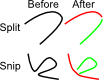
If what you really want is to just change the name of a
line for all of the slices in which it appears,
use , select a line,
select and specify a new name.
B in slices 10 to 15
should be considered to be a continuation of
line A that already appears in slices 5 to 9:
go to slice 10,
do ,
select line B, and then
select line A and specify
A
that appears in slices 5 to 15
needs to be treated differently in slices 10 to 15
than in slices 5 to 9: go to slice 10,
do ,
select line A,
then select
to create line B, and specify
Manual adjustment
Force weighting: ext,int = 0.6, 0.5
Pressure (e.g. 0.03) = 0.
Gradient/GVF = Gradient
Vertex spacing = 5.
Downsampling ratio = 1
Blurring (e.g. 1.) = 0.
Blue/Yellow thresholds = 19,inactive
Threshold strength (0.-1.) = 0.5
Image displayed = Original
Damping = 1.
Time step = 0.5
Open/Closed = Open
No. iterations = 100
Slither ahead
Undo & slither again
Restore original line
Quit
-
manual adjustment of nodes
when snake is having problems. Right-click in
the image window to reposition the currently
active node. (Do not try to use
the and
menu items, because
they are not properly implemented yet.)
! Zoom (don’t use)
@ Pan (don’t use)
Next point
Previous point
Delete point
Insert point
Append point
Trim all following points
Cut some following points
Quit
Each of these functions
first resamples the line only in the current slice, and then
offers the choices ,
and
.
If you select the last option,
it resamples the line in all of its slices with the same
settings.
It is often effective to use the median
filtering first, then averaging, and then spline fitting.
5.6.13 Delete lines
5.6.14 Locate lines
5.6.15 Modify lines
5.6.16 Transform z’s
5.6.17 Mark voxels
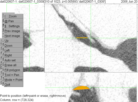
5.7 Stats
5.8 Tailor
 -
align the slices in a stack
by applying rotations
and translations. The main alignment display shows either
the current
image in shades of green overlaid on the previous image in
shades of red, or the contours in the current and previous
slices. Auxiliary windows display the contours in the previous,
current and next slice, and side views of the contours. The
current slice can be aligned manually by
(1) using Up, Down, Left, Right, Ccw (counterclockwise)
and Cw (clockwise) menu buttons, or
(2) using the mouse in the square control area,
with the inner portion causing translations and the outer portion
causing rotations (and ‘/’ as a shortcut key);
or by using
an automatic algorithm based on selected traced contours.
-
align the slices in a stack
by applying rotations
and translations. The main alignment display shows either
the current
image in shades of green overlaid on the previous image in
shades of red, or the contours in the current and previous
slices. Auxiliary windows display the contours in the previous,
current and next slice, and side views of the contours. The
current slice can be aligned manually by
(1) using Up, Down, Left, Right, Ccw (counterclockwise)
and Cw (clockwise) menu buttons, or
(2) using the mouse in the square control area,
with the inner portion causing translations and the outer portion
causing rotations (and ‘/’ as a shortcut key);
or by using
an automatic algorithm based on selected traced contours.
5.9 Quit
6. Model-definition file
6.1 Introduction
.tr3. These files are used by the Tr3
programme to create VRML and finite-element models.
Section
END?*
Notes
Comments
No
Any line starting with a semicolon is interpreted as a comment.
Only the comments at the beginning of the file, before the first
non-comment line, are preserved when Fie (or Tr3) saves a new
version of the file. Whenever Fie (or Tr3) saves a revised version
of the file, the user is asked for initials and a comment, which are
added (with the current date) to the
end of the initial comments.
LINES
Yes
See Lines
SCALE
No
See Scaling
XY_CALC
No
See Scaling
Z_CALC
No
See Scaling
SLICES
Yes
See Slices
JOINS
Yes
See Joins
CAPS
Yes
See Caps
SUBSETS
Yes
See Subsets
EXTERNAL
Yes
See External files
VOLUMES
Yes
See Volumes
MATERIALS
Yes
See Material properties
SPRINGS
Yes
See Springs
CONC_LOADS
Yes
See Concentrated loads
LABELS
Yes
See Labels
VIEWPOINTS
Yes
See Viewpoints
DATA
Yes
The actual x and y coördinates of lines
are stored in this section.
IMAGES
Yes
Definitions of images sets.
Seldom if ever used.
MARKED_VOXELS
Yes
Records marked voxels.
COSTS
Yes
Used by Tr3 to record cost functions chosen by user for triangulation.
Normally not directly modified by the user.
GLOBAL_RANGES
Obsolete
MERGES
Obsolete
END record.
[ ]) denote optional
elements and { | } denotes alternative values.
Roman (upright) characters denote actual strings to be used, while
italic (slanted) characters denote values to be chosen by the user.
6.2 Lines
LINES section of a .tr3 file,
the syntax for a line definition is:
name: [qualifiers] descriptive_text
-openclosed
{ OPEN | CLOSED }
-on
-off
-reverse
-do_slices
{ ALL | FIRST | LAST |
BOTH |
([zmin][,zmax]]) }
-colour
ecolour[;rcolour]
-transparency
transp
-boundary_condition
{ F |
C[{S|F|B|N}[{F|L|B}]]}
-pressure
press
-material
itype
-thickness
thick
-mtt
itype thick [deprecated]
-m
itype thick [deprecated]
-xyresolution
ires_xy
-zresolution
ires_z
-resolution
ires_xy ires_z [deprecated]
-linetype
{ STRAIGHT |
BEZIER |
ELLIPTICAL |
TUBING }
-start
[ ([[=]zmin][,
[=]zmax])]
{START|FINISH|NEAREST}
line_name
-finish
[ ([[=]zmin][,
[=]zmax])]
{START|FINISH|NEAREST}
line_name
-url
URL
-openclosed, -on and -off
all require at least two characters
after the hyphen (-).
Note that all attributes must start with a hyphen.
If you accidentally forget the hyphen, that attribute
and everything that follows it on the line will be treated as
descriptive text.
6.2.1 Basic attributes
mal_ and inc_, respectively. This makes
it easy to use wildcards in subset definitions.
Closed;
Fie will automatically join its last point to its first point.
Each end of an Open line can be connected to other lines using
the start-at and finish-at specifications
described below.
(There used to also be values of Filled,
Head, Tail and Both
but they are no longer used.)
6.2.2 Model-creation attributes
-on is not required because it is implied;
it will be overridden if -off is present.
-on is not implied,
even if one the following attributes is specified,
so it must be given explicitly if that is the intent.
If for some reason both -on and -off
are present in the same line definition or subset record,
whichever comes last will take effect.
-start is specified then the starting point
of the line is independent of any other line.
-start specification applies to all slices in which
the line being started at appears.
-start specification, and there
can be multiple -start specifications for a line.
A z range is specified by a zmin
and a zmax. If zmin
is not specified, it is taken to be equal to the
zmax of the previous -start
of the line, or to –∞
for the first -start.
If zmax is not specified, it is taken to be
equal to +∞. If zmin is preceded by
= then the -start applies for
zmin ≤ z; otherwise
it applies for
zmin < z.
Similarly, if zmax is preceded by
= then the -start applies for
z ≤ zmax; otherwise
it applies for
z < zmin.
If there are multiple -start specifications for
a line, then normally their z ranges should not overlap
and they should be arranged in order of increasing z.
In any case, when -start specifications are being
interpreted for a particular slice, the first one that matches
the z of the slice will be used.
If a line has both -start and
-finish specifications in a particular slice, then
the line will exist in that slice even if it has no points
of its own. It will be displayed as a thin line.
If a line has no points or only one point
of its own, it’s direction will be defined as running from
its start-at point to its finish-at point;
otherwise its own points determine its direction.
If a line has both -start and
-finish specifications,
sometimes it is necessary to explicitly specify the
z range to prevent a line from showing up in slices
where it is not intended.
Reasonable default values might be 50 for ires_xy, meaning that the triangle sizes will be approximately 1/50 of the estimated overall diameter of the model; and 1 for ires_z, meaning that every slice will be used in generating triangles. Values of, say, 10 and 3 would mean a coarser mesh, with only about 10 triangles across the diameter of the model and only using every 3rd slice. Different ires_xy and ires_z values can be used for different lines, although problems will arise from the use of different ires_z values for lines which are interconnected.
An x-y resolution of zero means that Tr3 will just use the points that it gets from Fie and will not generate new points by redividing lines to obtain any particular mesh resolution. This is particularly suitable for models used just for visualization and not for simulation. (For simulation, this option may be an easy way to obtain graded mesh resolutions but it sacrifices the ability to easily do mesh convergence studies by just changing the mesh-resolution parameters.)
In the case of tubing, ires_xy is interpreted as the number of sides of the polygon used to represent the circular cross-section of the tubing. The number of sides is constrained to the range 8 to 40, and if ires_xy = 0 then the number of sides is set to the default value of 8.
do_slices
by default has the value
ALL, which means that the line will be eligible
for triangulation in all slices in which it appears (subject
to the effects of the z resolution ires_z). If
do_slices has the value FIRST,
LAST or BOTH, then
only the first occurrence of the line, or only the last occurrence,
or both the first and last occurrences,
will be included in the triangulation process
(subject to the effects of ires_z).
This means that no triangles will be generated for the line itself,
but that it will be available for use in joins and caps.
(Using BOTH like this is a special case
in which Tr3 will not create a triangulated surface for a line
even though the line is present in more than one slice.)
do_slices can also specify a range of z values
enclosed in parentheses.
In this case triangles will be generated for the line.
If zmin is not specified
(indicated by a leading comma)
then the line will be included starting from its first slice,
while if zmax is not specified then
the line will be included until its last slice.
If do_slices is encountered more than once
in a line definition or subset record,
only the last one will take effect.
diprgb.txt file.
F | Free at all nodes |
C | Clamped at all nodes |
CS | Clamped at start node |
CSF | Clamped at start node and along all of first slice |
CSL | Clamped at start node and along all of last slice |
CSB | Clamped at start node and along all of first and last slices |
CF | Clamped at finish node |
CFF | Clamped at finish node and along all of first slice |
CFL | Clamped at finish node and along all of last slice |
CFB | Clamped at finish node and along all of first and last slices |
CB | Clamped at both ends |
CBF | Clamped at both ends and along all of first slice |
CBL | Clamped at both ends and along all of last slice |
CBB | Clamped at both ends and along all of first and last slices |
CNF | Clamped at neither end but along all of first slice |
CNL | Clamped at neither end but along all of last slice |
CNB | Clamped at neither end but along all of first and last slices |
Boundary conditions are specified for lines but are ultimately applied to nodes of finite-element models.
F means that no nodes on this particular line are clamped,
while C alone means that all nodes on this line
are clamped in all slices.
C can also be followed by one or two
qualifiers.
For the first qualifier: S means that
only the start node of the line is clamped (in all slices),
F means that only the finish node is clamped, and
B means that both the start and finish nodes are clamped
but not the rest of the line.
(N means that none of the line is clamped in all slices
and it is used only in combination with the second qualifier.)
For the second qualifer: F means that (in addition to
whatever clamping is specified by the first qualifier)
all nodes on the first slice are clamped,
L means that all nodes on the last slice are clamped, and
B means that all nodes on both the first and last
slices are clamped.
MATERIALS
section of the file
incus1: -op CL -c yellow;bone -r 100 1 -m 1 .04 ;Incus top
|
incus1 demonstrates a closed line which will be shown as
yellow in Fie and rendered as bone coloured in the 3-D models; which
is to be triangulated using every slice at 100 elements/diameter; and
which consists of material type 1 with a thickness of 0.04.
tm_inf: -op OP -c green;white -t .5 -r 50 2 -m 4 .001 -s f annlig -f s manub ;TM
|
tm_inf demonstrates an open line which will be shown
as green in Fie, but in the VRML model as translucent white with a
transparency of 0.5; it is to be triangulated using only every second
slice at 50 elements/diameter; it consists of material type 4 with
a thickness of 0.001; and it starts at the finish of line annlig
and finishes at the start of line manub.
The first line of the SLICES section may be of the form
IMAGE_PATH path
|
path can be used to specify where to find the image files if they are not in the same directory as the .tr3 file. It will be prefixed to the image names before the path of the .tr3 file is prefixed, so it will specify a path relative to the path of the .tr3 file. (Neither the image-path name nor the path of the .tr3 file will be used if the image name itself contains a path specification.) The image-path name should not include leading or trailing path delimiters; it will be system independent if it does not include any path delimiters, i.e., it specifies only a single directory name. This path is used only when there is a separate image file for each slice. The usual method is to put all of the image files into a subdirectory of the directory where the .tr3 file is, and then give the subdirectory name as the path.
The rest of the SLICES section consists of records of the form
i, name, [z, [rotate, offsetx, offsety]]
|
There should be one record for each image (slice). i is the slice sequence number. name is a descriptive name for the slice (or an actual file name when the slices are stored as separate files). z is the z coördinate for the slice. rotate, offsetx and offsety optionally specify the offset and orientation required to align the image with the rest of the stack (usually for histological images).
As a structure subdivides from slice to slice, or becomes connected to other structures, multiple line names must be used for the same structure. By default, Tr3 only triangulates across slices between lines that have the same name. Therefore, the Join mechanism is provided to specify how triangulation should be done when line names change. The syntax for Joins allows concatenation of multiple lines; forward or backward traversal of lines; and incorporation of only the first or last point of a line. The syntax permits transitions between Closed and Open lines. Joins can either inherit properties from the lines which constitute them, or take on new properties.
Within the JOINS section of a .tr3 file,
the syntax for a Join definition is:
name: [qualifiers]
	[-]i1[{>|<}] [-]i2[{>|<}] … to
	[-]j1[{>|<}] [-]j2[{>|<}] …
	[;description]
|
i1, i2, etc., are the names of the lines to be concatenated in order to form multiline 1. j1, j2, etc., are the names of the lines to be concatenated in order to form multiline 2. A surface is triangulated between multiline 1 and multiline 2. Multiline 1 should be in a lower-numbered slice than multiline 2.
A minus sign (-) before a
line name means that that line is to be traversed backwards when being
concatenated to its multiline.
The symbol > after a
line name means that only the first node of that line is used.
The symbol < after a
line name means that only the last node of that line is used.
The following attributes (qualifiers) can be defined for Joins. Their meanings are the same as for line attributes.
Example. If you had a structure defined by
two open lines, bone_ant_50 and bone_post_50,
from slices 50 to 79, and then at slice 80 they combined into a
single closed line,
bone_80, you could define the join
between them as
bone_50: bone_ant_50 bone_post_50 to bone_80 ;Bone
|
If you wanted to specify a distinctive colour for the triangles corresponding to the join, you could use, for example,
bone_50: -c red bone_ant_50 bone_post_50 to bone_80 ;Bone
|
Within the CAPS section of a .tr3 file,
the syntax for a Cap definition is:
name: {HEAD|TAIL} [qualifiers]
	[-]i1[{>|<}] [-]i2[{>|<}] …
	[;description]
|
HEAD means that the cap is to created at the first slice
for which all of the component lines are present.
TAIL means that the cap is to created at the last slice
for which all of the component lines are present.
i1, i2, etc., are the names of the lines to be concatenated in order to form the cap. A flat surface is triangulated within the resulting multiline.
A minus sign (-) before a
line name means that that line is to be traversed backwards when being
concatenated to the multiline.
The symbol > after a
line name means that only the first node of that line is used.
The symbol < after a
line name means that only the last node of that line is used.
The following attributes (qualifiers) can be defined for Caps. Their meanings are the same as for line attributes.
F and C are the only
accepted values, and they apply only to the internal nodes
of the cap
Example. If you had a structure defined by
two open lines, bone_ant_50 and bone_post_50,
from slices 50 to 79, you could a define a cap at slice 50 as
bone: HEAD bone_ant_50 bone_post_50 ;Bone
|
bone: TAIL bone_ant_50 bone_post_50 ;Bone
|
The syntax for the VOLUMES section of a .tr3 file
is the following:
| ||||||||||||||||||||||||||||||||||||||
i1, i2, etc., are the names of the lines to be concatenated in order to form a closed multiline. These closed multilines should be specified in the order in which they are encountered in processing from the first slice to the last.
The syntax for specifying a multiline is the same as for Joins and Caps.
A minus sign (-) before a
line name means that that line is to be traversed backwards when being
concatenated to the multiline.
The symbol > after a
line name means that only the first node of that line is used;
the symbol < after a
line name means that only the last node of that line is used.
The purpose of this section is to produce surface
model definitions suitable for use by volume-mesh generators.
This section has essentially been superseded by the use of the
Volume qualifier for subsets.
The syntax of the SUBSETS section of a .tr3 file
is the following:
| ||||||||||||||||||||||||||||||||||||||
A subset name may contain only letters (a-z, A-Z), digits (0-9), and '_'.
The optional VOLUME qualifier is obsolete.
It was intended to result in the
output of the model in file formats for use by volume-mesh
generators, but
currently no such formats are output because a separate application
(Fad)
is used to convert .sap files
to Gmsh format.)
This qualifier
was to be used only for a subset which defines a single, simple closed
surface.
The optional MIRROR qualifier causes the model to
be flipped to become a mirror image: the z coördinates
are all multiplied by –1 and the node numbering is reversed in each
triangle. It may be a good idea to add _mirror or some other
indicator to the name of the subset.
The syntax for each subset record is one of the following:
      linename: [qualifiers]
					descriptive_text
|
      (cap) capname: [qualifiers]
					descriptive_text
|
      (join) joinname: [qualifiers]
					descriptive_text
|
(label) labelname: { -on | -off }
|
(spring) springname: { -on | -off }
|
(concload) loadname: { -on | -off }
|
(vol) volname: { -on | -off }
|
      (clip) { xmin val | xmax val |
	       xrange val1 val2 |
	       ymin val | ymax val |
	       yrange val1 val2 |
	       zmin val | zmax val |
	       zrange val1 val2 }
|
      (rot) θx θy
		 θz
|
(tran) tx ty tz
|
@[-]subsetname
|
SUBSETS
| ||
SUBSET Bone
| ||
*: -off
| ||
bone*: -on -c red
| ||
(join) bone1: -off
| ||
(join) bone2: -on
| ||
End of subset
| ||
End of subsets
| ||
Each line, cap and join name field can contain any number
of the wildcard characters
* and ?. The
* matches any number of characters, including zero
characters, and the ? matches exactly one character.
For example, inc?_*med_* would match
incA_antmed_050,
incB_postmed_100, etc.
This works best if
lines are named systematically.
Any of the line, cap and join attributes which are specified here
will over-ride those specified in the original line, cap and join
definitions. In the case of -reverse used for caps and joins
in a subset definition, it will cause the current setting to be flipped.
For the new attributes to take effect, -on must be specified
explicitly.
The (label), (spring),
(concload) and (vol) lines are used to turn
specified labels, springs, concentrated loads and volumes on or off.
The (clip) line is used to exclude ranges
of x and y, or slices
based on their z values, from the 3-D model. For example,
(clip) zmin 5. would cause all slices with z
less than 5. to be dropped;
(clip) zmax 10. would cause all slices with z
greater than 10. to be dropped; and
(clip) zrange 5. 10. would result in keeping
only slices with 5. ≤ z ≤ 10.
The (rot) and (tran) lines are used to
apply specified rotations and translations to the overall model.
The @ line is used to include another subset
within this subset. Subsets can be nested to any depth; that is,
the included subset can itself include other subsets.
The optional - (minus sign) can
be used to reverse the numbering of all of the triangles in the
included subset.
The usual practice is to begin each subset definition with
*: -off (i.e., turn off all lines) and then turn on
the desired lines, turn caps and joins on or off as required,
etc. When some other subset is included using an @ line,
the *: -off line of the included subset is ignored
(to avoid turning off the lines that have already been turned on in
the subset requesting the inclusion).
As an example, the SUBSET definition shown on the right would suppress all
lines and then reactivate (and turn red) all those whose names start
with ‘bone’. It would also turn off Join bone1
and replace it with join bone2 (which presumably would
initially have been defined with -off.
Within the MATERIALS section of a .tr3 file,
the syntax for a record is:
      nmat ym pr den
					descriptive_text
|
nmat is a sequence number for the material type, normally starting at 1 and incremented for each material type. ym is the Young’s modulus, pr is Poisson’s ratio, and den is the mass density of the material. The value of the Young’s modulus may be expressed with a metric prefix added after the number (with no space); for example, 2G or 2.G for 2 GPa, or 1.5M for 1.5 MPa.
Everything after the density value is taken as descriptive text.
If no material properties are defined, then no .sap finite-element model will be generated by Tr3.
Within the SPRINGS section of a .tr3 file,
the syntax for a record is:
	{D|R} stiffness [-off]
	      node0 node1
	      [node2 [node3 [node4]]]
|
	{D|R} stiffness [-off] -xyz
	      node0 x,y,z
|
If the first item in the spring definition is D
then the spring is a translational one (e.g., N/m);
if it’s an R then the spring is a
rotational one (e.g., N/rad).
stiffness is the actual stiffness
of the spring. The rest of the record defines from 1 to 5 nodes.
Each node is defined by a line name, an optional z value, and an optional fraction f from 0 to 1:
line[([z][,
|
The spring will be attached to the model at node 0.
The direction of the spring is determined by the position(s) of the
other nodes, as described in the following table.
The notation Vmn indicates a vector from node m to
node n.
| No. other nodes | Direction of spring |
|---|---|
| 1 | parallel to V01 |
| 2 | parallel to V12 |
| 3 | perpendicular to the plane formed by V12 and V13 |
| 4 | perpendicular to the plane formed by V12 and V34 |
The position of the other (unattached) end of the spring can also be
specified by its x, y and z coordinates
by using the -xyz option.
Note that the length of the spring doesn’t matter.
Within the CONC_LOADS section of a .tr3 file,
the syntax for a record is:
	{F|M} load
	      node0 node1
	      [node2 [node3 [node4]]]
|
If the first item in the concentrated-load definition is F
then the load is a force (e.g., N);
if it’s M then the load is a
moment (torque, e.g., N m).
load is the actual value
of the load.
The nodes are defined in the same way as for springs.
The load will be applied to the model at node 0
and the direction of the load is determined in the same way as for springs.
The -xyz option is not yet available for concentrated loads.
Within the LABELS section of a .tr3 file,
the syntax for a record is:
	label_text [-size size]
	[-colour colour]
	[-family family]
	node0 [node1]
|
label_text is the text that will be displayed as the
label. If the text contains any space characters, it should be enclosed
in double quotation marks, e.g., "Label 1".
size is the font size used for the label, measured in the same units as the model. If unspecified, the default value is 1. If the specified size is negative, no text will be displayed and the label may be interpreted as a pin head.
colour is the colour used for the text of the label, specified by name. If unspecified, the default value depends on the browser. The colour names available are the same as those offered by menu as line, join and cap colours.
family specifies the font family to be used
for the label. It can specify the name of any font on the user’s
computer, but the only values guaranteed to work are the generic
values SERIF, SANS
and TYPEWRITER.
If unspecified, the default value is SERIF.
The label (in particular, at least in some viewers, the lower left corner of the first character of the label’s text) will be located at node 0, and the label will be attached to the model by a line running to node 1, if defined.
If the font size is negative then the label itself will not appear. It may be rendered as a pin head in some viewers.
Viewpoints cannot yet be defined
using Fie’s graphical interface.
Thrwp’ny considers only the first viewpoint
and then only sets a view along either the +y
or −y axis, depending on whether there is
an asterisk in the viewpoint name or not.
Within the VIEWPOINTS section of a .tr3 file,
the syntax for a record is one of the following:
	name XYZ rotx roty rotz
		description
|
	name AA posx posy posz
		axisx axisy axisz angle
		description
|
(reldist) relative_distance
|
The xyz option defines a viewpoint corresponding to what
one sees in Fad after the specified x, y and
z rotations (in that order). In other words, one can use
the rotation angles displayed in Fad in order to re-create a
view from the same direction.
If one is starting from an orientation in
Thrup’ny, one can use
to display the rotation angles, apply them in the order z,
y and x in Fad using the interactive rotation
tool, and then use the angles displayed
by Fad.
The aa option defines a viewpoint using the same method
used by VRML itself. The required parameters can be determined by
requesting Tr3 to include code in the VRML file which causes the
current position
(posx posy posz) and
orientation
(axisx axisy axisz angle)
of the viewpoint to be continuously
displayed.
(This display doesn’t work in Thrup’ny.)
Whether or not any viewpoints are defined in the .tr3 file, six standard viewpoints are generated, in both directions along each of the x, y and z axes.
A (reldist) line defines the relative distance from the
centre of the model to any xyz-type viewpoint and
to the six standard viewpoints along the axes. The actual distance
is the relative distance multiplied by an estimate of the size of the model.
The default value for the relative distance is 2.
Fie needs to handle two different ways of thinking about x, y and z coördinates. On the one hand, line nodes need to be positioned with respect to pixel positions (columns and rows) within images and with respect to slice numbers within a stack of images. On the other hand, the x, y and z coördinates of the final model normally need to be expressed in real-world coördinates, e.g., millimetres.
There are two ways to manage Fie’s scaling between the real-world x, y and z coördinates of a model and the row, column and slice positions:
XY_CALC and Z_CALC parameters
to map the real-world coördinates
to pixel positions and slice numbers when displaying lines; or
SCALE parameters
to convert to real-world coördinates when creating the
final triangulated models.
XY_CALC
|
ux and uy are scaling parameters (in units/pixel). ox and oy are offsets (in pixels). These parameters are used by Fie to transform real-world x and y coördinates in the .tr3 file to match the images. The z coördinates of the slices are assumed to be given using the same real-world coördinates.
The directive XY_CALC is on one line and the parameter values
are on the next line.
By default, ux and uy are 1., and ox and oy are 0., implying that the x and y coördinates in the .tr3 file, and presumably also the z coördinates, are measured in pixels. If the z coördinates were measured in, say, mm, then ux and uy would normally specify the pixel size in mm.
If uy is not specified, it is assumed to be the same as ux, i.e., the x and y units are assumed to be the same.
The -u parameter is an optional name for the units, e.g.,
-u m for metres, or -u um for micrometres.
Example. If you had images with a pixel size of 0.5 mm, then you might use the following:
XY_CALC
|
Z_CALC
|
z1 is the z coördinate for the first image of a stack of images, measured in the same units as used for x and y. dz indicates the nominal spacing between slices.
The directive Z_CALC is on one line and the parameter values
are on the next line.
Note that these parameters are just used to guess an appropriate z coördinate for a slice which has not yet had a z coördinate assigned, and to assign slice numbers to contours read from an old .tr3 file which does not contain explicit slice-number/z-coördinate information.
If a .tr3 file currently uses pixels for its coördinates and you want to start using real-world coördinates, do the following:
m for metres,
mm for millimetres or um for
micrometres. Finally, answer
in response to the question about applying the transformation
to clipping.SCALE parameters if they are something
other than 1.0. (At the moment these parameters can only be
examined and modified using a text editor on the .tr3 file,
but they should always be 1.0 unless you are dealing with
an old .tr3 file created by someone else.)
SCALE
|
These scaling parameters are not actually used within Fie. Tr3 uses them to scale the x, y and z coördinates that it reads from the .tr3 file.
Normally only sx needs to be specified, and sy and sz will be taken to be the same as sx. By default, sx = 1.
The directive SCALE is on one line and the parameter values
are on the next line.
One use for these parameters is to produce real-world coördinates in the VRML and SAP files produced by Tr3 when the coördinates in the .tr3 file are expressed in pixels.
Example. If you had images with a pixel size of 0.5 mm, then you might use the following:
SCALE
|
The SCALE parameters could also be used to convert from
one set of units to another, say from mm in
the .tr3 file to m in the VRML and SAP files.
On the right is a partial screenshot that includes 3 of Fie’s windows. Click on the screenshot for a larger version.
The main window shows part of slice 127 from magnetic-resonance microscopy dataset 516871 for a cat middle ear. The data are courtesy of Drs. O.W. Henson, Jr. and Miriam M. Henson (UNC) and the CIVM (Duke University). The image shown is a small part of the original MR image.
Below the main image window are x-z and z-y views showing a selected subset of the lines that have been created by the user. The lines shown in the side views correspond to parts of the eardrum, malleus, tensor tympani muscle and stapes.
Each line in the image is represented by a set of vertices. The first vertex of a line is represented by a rightward-pointing triangle; the last vertex is represented by a leftward-pointing triangle; and the others are represented by squares. The straight-line segments between the vertices of a line are relatively thick. When a line is specified as starting at, or finishing at, some other line, then that connection is drawn as a thin straight-line segment.
In the centre of the image are seen a part of the malleus bone (yellow) and
the tensor tympani muscle (red) attached to it. Notice that the shared surface
between the two is represented as a separate line. These lines could be
defined as shown in the following table: mallmuscinf
and mallmuscsup represent the inferior (lower) and superior
(upper) lines defining the part of the malleus to which the muscle is
attached, and ttymp represents the tensor tympani muscle.
The lines mallmuscsup and ttymp are both
defined as starting at the finish of mallmuscinf and
finishing at the start of mallmuscinf. Note that the bone
has a material type of 1 while the muscle has a material type of 2.
mallmuscinf: -op OP -c yellow;bone -xyr 100 -mat 1 Malleus
|
mallmuscsup: -op OP -c yellow;bone -xyr 100 -mat 1 -s f mallmuscinf -f s mallmuscinf Malleus
|
ttymp: -op OP -c red;muscle -xyr 100 -mat 2 -s f mallmuscinf -f s mallmuscinf Tensor tympani
|
 AudiLab home page